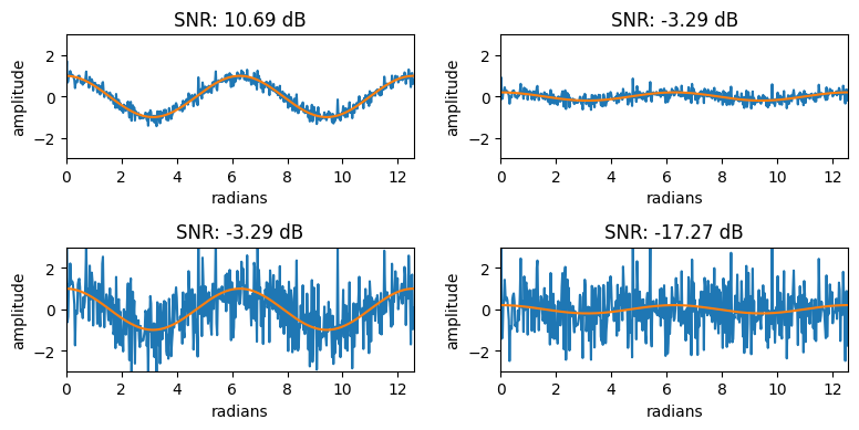
Signal and noise#
Any measured signal may be tainted by noise.
Recovering the true signal may be impossible.
However, we will look at some methods use various strategies for
suppressing noise,
estimating derivatives,
decomposing into different frequencies,
decomposing into trend, seasonal changes and residual, and
exploratory data analysis.
Signal-to-Noise Ratio (SNR)#
Signal-to-noise is a ratio that can be caulculated in various ways.
A measure of how easy it is to extract the underlying information.
A common definition is decibel (dB) based.
0 decibel means the signal and noise are of equal magnitude.
Every 10 decibel increase means 10 times higher power of the signal compared to the noise.
Example: HiFi amplifier:
>100 dB SNR, i.e., \(10^{10}\) times higher power of the signal than the noise.
\(SNR = 10 \cdot log_{10} \frac{\sum s_i^2}{\sum n_i^2}\), where \(s\) is the signal and \(n\) is the noise.
If the true signal and noise are lost, estimates of these can be made.
import numpy as np
def SNR(signal, noise):
    return 10*np.log10(np.sum(signal**2)/np.sum(noise**2))
# Plot a cosine curve from 0 to 4pi
import matplotlib.pyplot as plt
import numpy as np
x = np.linspace(0, 4*np.pi, 500)
y_cos = np.cos(x)
noise = 0.2*np.random.normal(size=(len(x)))

# Plot the cosine curve with noise
sig = [1, 0.2]
noi = [1, 5]
plt.figure(figsize=(8, 4))
for i in range(4):
    plt.subplot(221+i)
    plt.plot(x, y_cos*sig[np.mod(i,2)] + noise*noi[i//2], label='Noisy cosine curve')
    plt.plot(x, y_cos*sig[np.mod(i,2)], label='Cosine curve')
    plt.xlabel('radians')
    plt.ylabel('amplitude')
    plt.title('SNR: {:.2f} dB'.format(SNR(y_cos*sig[np.mod(i,2)], noise*noi[i//2])))
    plt.xlim((0,4*np.pi))
    plt.ylim((-3,3))
#    plt.legend()
plt.tight_layout()
plt.show()


