This is a quite general and flexible implementation of APLS.
Usage
apls(
  formula,
  data,
  add_error = TRUE,
  contrasts = "contr.sum",
  permute = FALSE,
  perm.type = c("approximate", "exact"),
  ...
)
Arguments
- formula
Model formula accepting a single response (block) and predictors. See Details for more information.
- data
The data set to analyse.
- add_error
Add error to LS means (default = TRUE).
- contrasts
Effect coding: "sum" (default = sum-coding), "weighted", "reference", "treatment".
- permute
Number of permutations to perform (default = 1000).
- perm.type
Type of permutation to perform, either "approximate" or "exact" (default = "approximate").
- ...
Additional arguments to
hdanova.
Value
An apls object containing loadings, scores, explained variances, etc. The object has
associated plotting (asca_plots) and result (asca_results) functions.
Details
APLS is a method which decomposes a multivariate response according to one or more design
variables. ANOVA is used to split variation into contributions from factors, and PLS is performed
on the corresponding least squares estimates, i.e., Y = X1 B1 + X2 B2 + ... + E = T1 P1' + T2 P2' + ... + E.
For balanced designs, the PLS components are equivalent to PCA components, i.e., APLS and APCA are equivalent.
This version of APLS encompasses variants of LiMM-PLS, generalized APLS and covariates APLS.
The formula interface is extended with the function r() to indicate random effects and comb() to indicate effects that should be combined. See Examples for use cases.
References
Smilde, A., Jansen, J., Hoefsloot, H., Lamers,R., Van Der Greef, J., and Timmerman, M.(2005). ANOVA-Simultaneous Component Analysis (ASCA): A new tool for analyzing designed metabolomics data. Bioinformatics, 21(13), 3043–3048.
Liland, K.H., Smilde, A., Marini, F., and Næs,T. (2018). Confidence ellipsoids for ASCA models based on multivariate regression theory. Journal of Chemometrics, 32(e2990), 1–13.
Martin, M. and Govaerts, B. (2020). LiMM-PCA: Combining ASCA+ and linear mixed models to analyse high-dimensional designed data. Journal of Chemometrics, 34(6), e3232.
See also
Main methods: asca, apca, limmpca, msca, pcanova, prc and permanova.
Workhorse function underpinning most methods: hdanova.
Extraction of results and plotting: asca_results, asca_plots, pcanova_results and pcanova_plots
Examples
# Load candies data
data(candies)
# Basic APLS model with two factors
mod <- apls(assessment ~ candy + assessor, data=candies)
print(mod)
#> Anova Partial Least Squares fitted using 'lm' (Linear Model)
#> Call:
#> apls(formula = assessment ~ candy + assessor, data = candies)
# APLS model with interaction
mod <- apls(assessment ~ candy * assessor, data=candies)
print(mod)
#> Anova Partial Least Squares fitted using 'lm' (Linear Model)
#> Call:
#> apls(formula = assessment ~ candy * assessor, data = candies)
# Result plotting for first factor
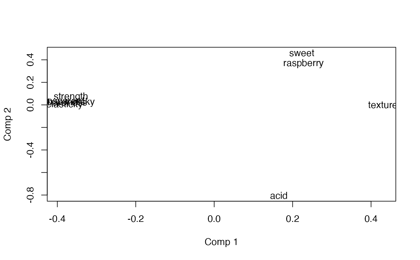
loadingplot(mod, scatter=TRUE, labels="names")
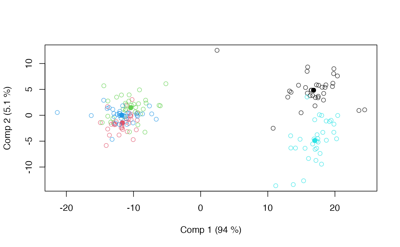
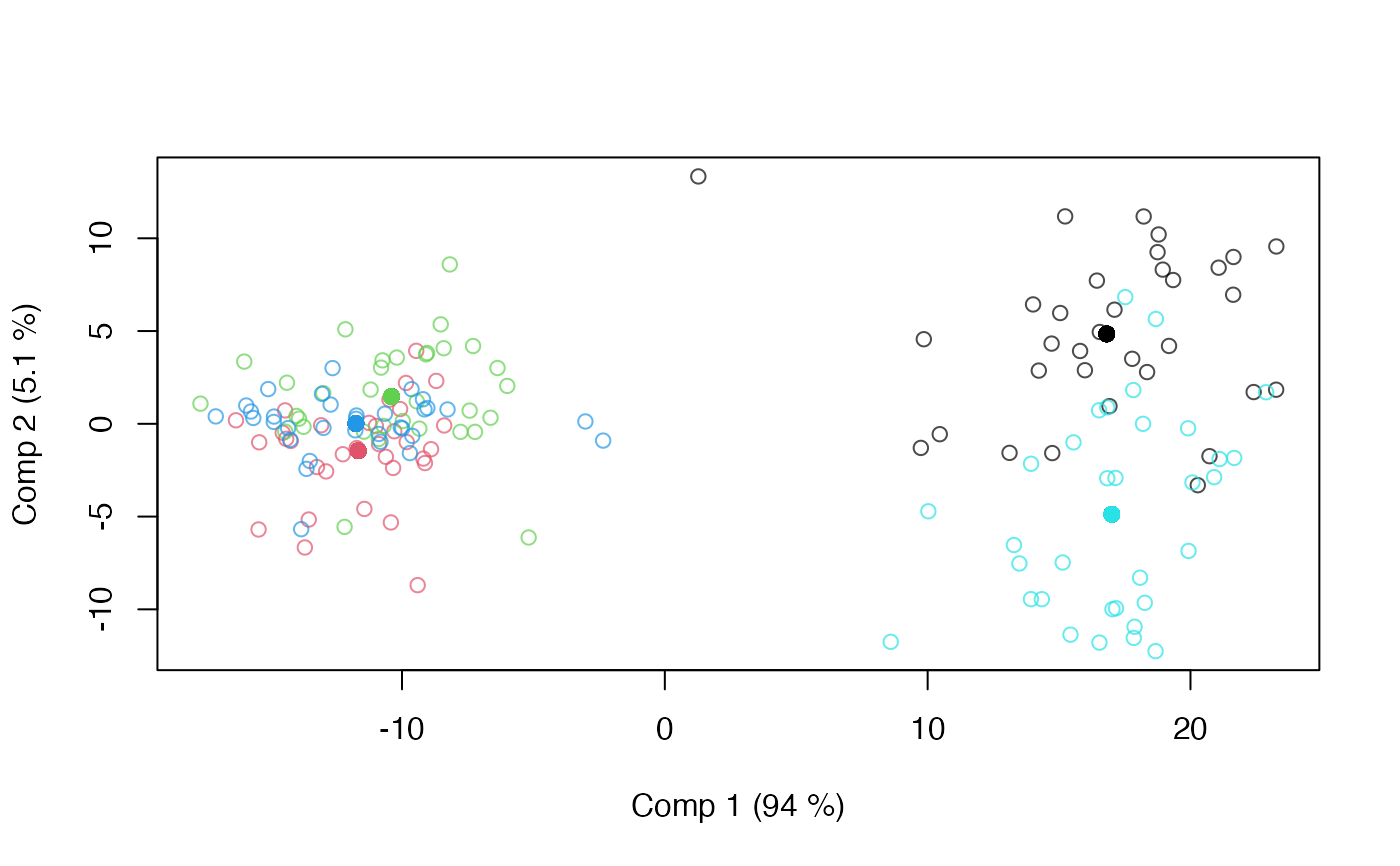
 scoreplot(mod)
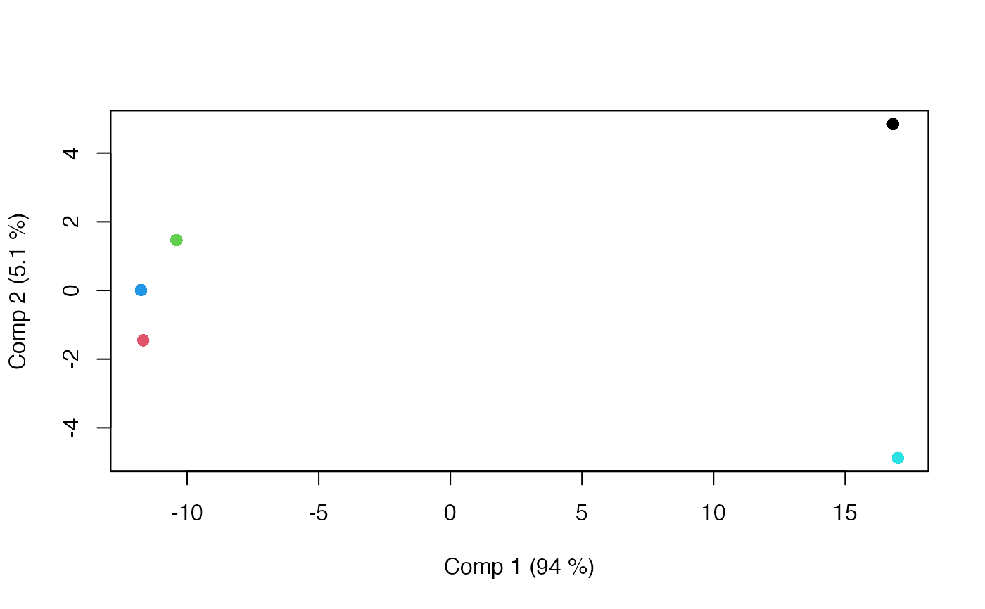
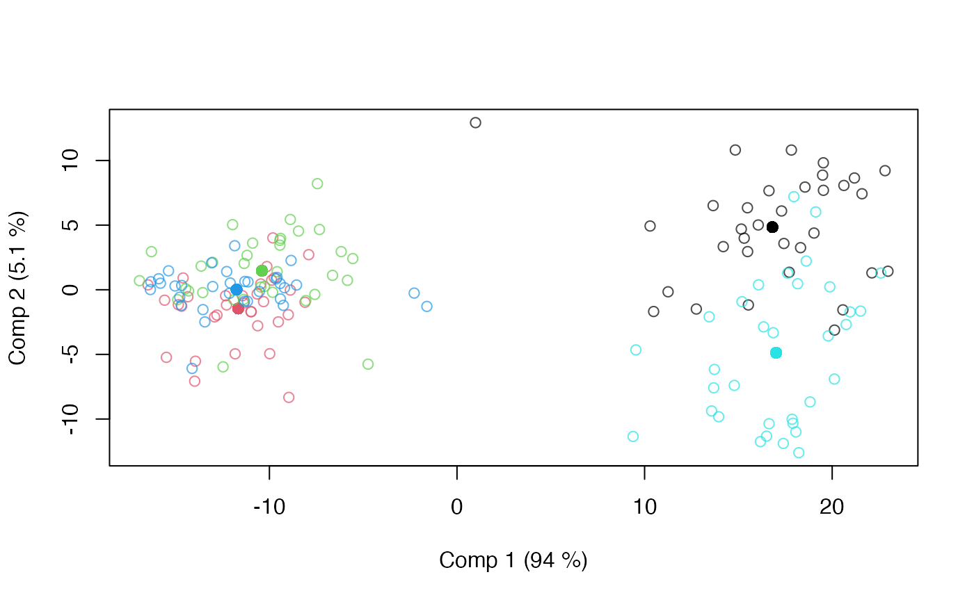
 # No backprojection
scoreplot(mod, projections=FALSE)
# No backprojection
scoreplot(mod, projections=FALSE)
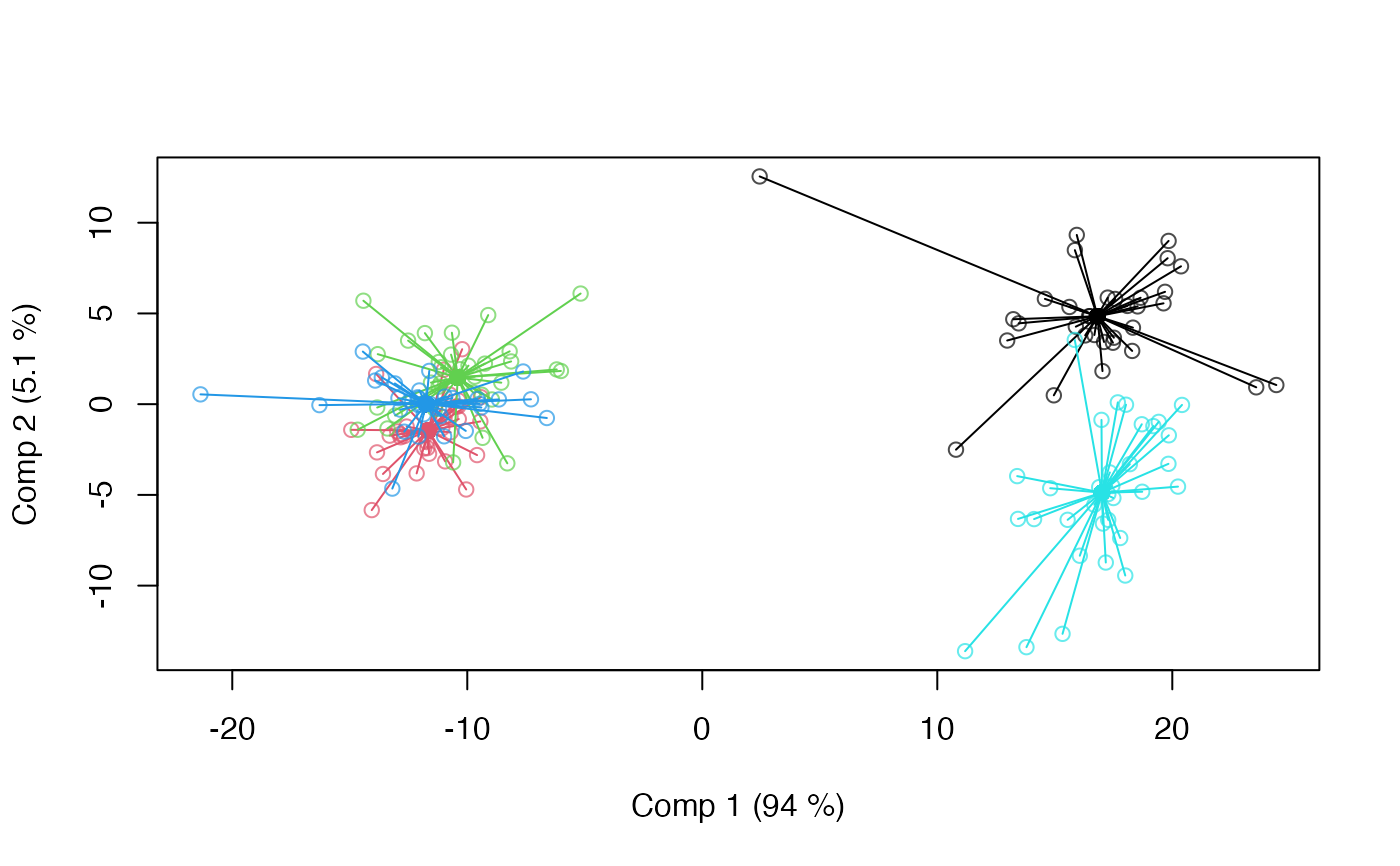
 # Spider plot
scoreplot(mod, spider=TRUE)
# Spider plot
scoreplot(mod, spider=TRUE)
 # APLS model with compressed response using 5 principal components
mod.pca <- apls(assessment ~ candy + assessor, data=candies, pca.in=5)
# Mixed Model APLS, random assessor
mod.mix <- apls(assessment ~ candy + r(assessor), data=candies)
scoreplot(mod.mix)
# APLS model with compressed response using 5 principal components
mod.pca <- apls(assessment ~ candy + assessor, data=candies, pca.in=5)
# Mixed Model APLS, random assessor
mod.mix <- apls(assessment ~ candy + r(assessor), data=candies)
scoreplot(mod.mix)
 # Mixed Model APLS, REML estimation
mod.mix <- apls(assessment ~ candy + r(assessor), data=candies, REML=TRUE)
scoreplot(mod.mix)
# Mixed Model APLS, REML estimation
mod.mix <- apls(assessment ~ candy + r(assessor), data=candies, REML=TRUE)
scoreplot(mod.mix)
 # Load Caldana data
data(caldana)
# Combining effects in APLS
mod.comb <- apls(compounds ~ time + comb(light + time:light), data=caldana)
summary(mod.comb)
#> Anova Partial Least Squares fitted using 'lm' (Linear Model)
#> - SS type II, sum coding, restricted model, least squares estimation, SSQ method: qr_regression
#> Sum.Sq. Expl.var.(%)
#> time 154.58 9.69
#> light+time:light 349.64 21.92
#> Residuals 1091.14 68.39
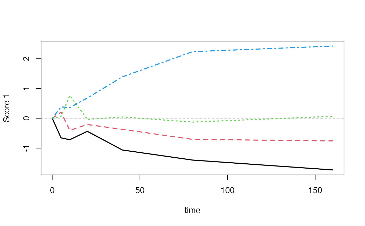
timeplot(mod.comb, factor="light", time="time", comb=2)
# Load Caldana data
data(caldana)
# Combining effects in APLS
mod.comb <- apls(compounds ~ time + comb(light + time:light), data=caldana)
summary(mod.comb)
#> Anova Partial Least Squares fitted using 'lm' (Linear Model)
#> - SS type II, sum coding, restricted model, least squares estimation, SSQ method: qr_regression
#> Sum.Sq. Expl.var.(%)
#> time 154.58 9.69
#> light+time:light 349.64 21.92
#> Residuals 1091.14 68.39
timeplot(mod.comb, factor="light", time="time", comb=2)
 # Permutation testing
mod.perm <- apls(assessment ~ candy * assessor, data=candies, permute=TRUE)
summary(mod.perm)
#> Anova Partial Least Squares fitted using 'lm' (Linear Model)
#> - SS type II, sum coding, restricted model, least squares estimation, SSQ method: qr_regression, 1000 permutations
#> Sum.Sq. Expl.var.(%) p-value
#> candy 33416.66 74.48 0
#> assessor 1961.37 4.37 0
#> candy:assessor 3445.73 7.68 0
#> Residuals 6043.52 13.47 NA
# Permutation testing
mod.perm <- apls(assessment ~ candy * assessor, data=candies, permute=TRUE)
summary(mod.perm)
#> Anova Partial Least Squares fitted using 'lm' (Linear Model)
#> - SS type II, sum coding, restricted model, least squares estimation, SSQ method: qr_regression, 1000 permutations
#> Sum.Sq. Expl.var.(%) p-value
#> candy 33416.66 74.48 0
#> assessor 1961.37 4.37 0
#> candy:assessor 3445.73 7.68 0
#> Residuals 6043.52 13.47 NA