Linear Mixed Model PCA

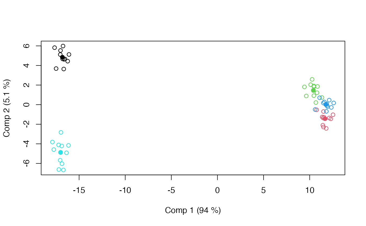
This function mimics parts of the LiMM-PCA framework, combining ASCA+ and linear mixed models to analyse high-dimensional designed data. The default is to use REML estimation and scaling of the backprojected errors. See examples for alternatives.

Usage

limmpca(
  formula,
  data,
  pca.in = 5,
  aug_error = 0.05,
  use_ED = FALSE,
  REML = TRUE,
  contrasts = "contr.sum",
  permute = FALSE,
  perm.type = c("approximate", "exact"),
  SStype = "III",
  ...
)

Arguments

formula

Model formula accepting a single response (block) and predictors. See Details for more information.

data

The data set to analyse.

pca.in

Compress response before ASCA (number of components), default = 5.

aug_error

Error term of model ("denominator", "residual", numeric alpha-value). The latter implies the first with a scaling factor.

use_ED

Use Effective Dimensions instead of degrees of freedom when scaling.

REML

Use restricted maximum likelihood estimation. Alternatives: TRUE (default), FALSE (ML), NULL (least squares).

contrasts

Effect coding: "sum" (default = sum-coding), "weighted", "reference", "treatment".

permute

Number of permutations to perform (default = 1000).

perm.type

Type of permutation to perform, either "approximate" or "exact" (default = "approximate").

SStype

Type of sum-of-squares: "I" = sequential, "II" = last term, obeying marginality, "III" (default) = last term, not obeying marginality.

...

Additional arguments to hdanova.

Value

An object of class limmpca, inheriting from the general asca class.

Details

The Sum of Squares for the model is dependent on the SStype of the model. For SStype = "I" and SStype = "II" the SSQ is based on LLR (possibly inflating large contributions), while it is directly estimated from the model for SStype = "III". SStype = "III" is the default for LiMM-PCA and should be combined with sum coding. Sum of Squares for the random effects are based on the variance components.

References

• Martin, M. and Govaerts, B. (2020). LiMM-PCA: Combining ASCA+ and linear mixed models to analyse high-dimensional designed data. Journal of Chemometrics, 34(6), e3232.

See also

Main methods: asca, apca, limmpca, msca, pcanova, prc and permanova. Workhorse function underpinning most methods: hdanova. Extraction of results and plotting: asca_results, asca_plots, pcanova_results and pcanova_plots

Examples

# Load candies data
data(candies)

# Default LiMM-PCA model with two factors and interaction, 5 PCA components
mod <- limmpca(assessment ~ candy*r(assessor), data=candies)
summary(mod)
#> LiMM-PCA fitted using 'lmm' (Linear Mixed Model) 
#> - SS type III, sum coding, restricted model, REML estimation 
#>                 Sum.Sq. Expl.var.(%)
#> candy          33394.40        78.00
#> candy:assessor  1192.09         2.78
#> assessor         968.07         2.26
#> Residuals       7257.45        16.95
scoreplot(mod, factor = "candy")


# LiMM-PCA with least squares estimation and 8 PCA components
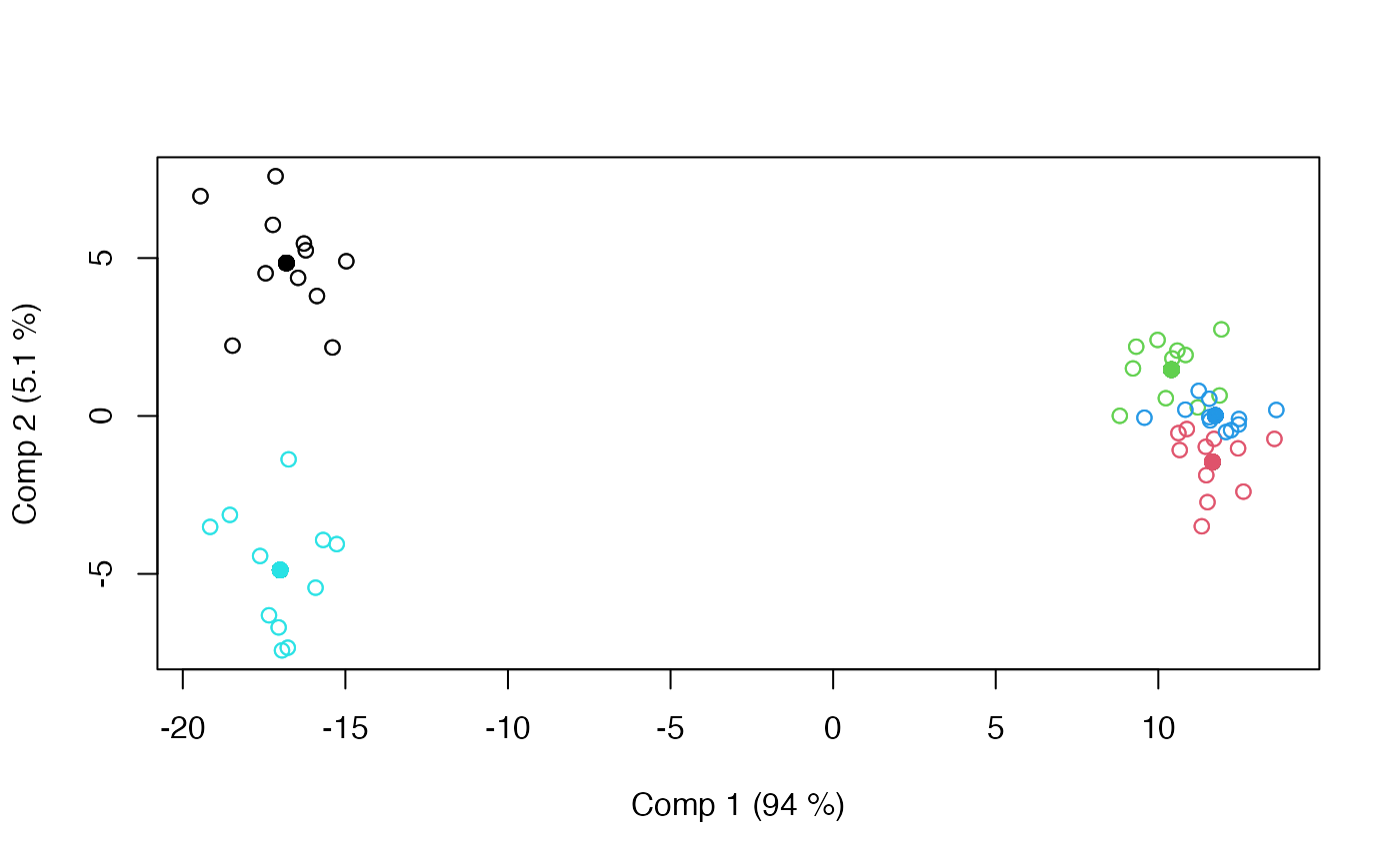
modLS <- limmpca(assessment ~ candy*r(assessor), data=candies, REML=NULL, pca.in=8)
summary(modLS)
#> LiMM-PCA fitted using 'lmm' (Linear Mixed Model) 
#> - SS type III, sum coding, restricted model, least squares estimation 
#>                 Sum.Sq. Expl.var.(%)
#> candy          33415.98        74.73
#> assessor        1948.75         4.36
#> candy:assessor  3419.04         7.65
#> Residuals       5934.46        13.27
scoreplot(modLS, factor = "candy")


# Load Caldana data
data(caldana)

# Combining effects in LiMM-PCA (assuming light is a random factor)
mod.comb <- limmpca(compounds ~ time + comb(r(light) + r(time:light)), data=caldana, pca.in=8)
summary(mod.comb)
#> LiMM-PCA fitted using 'lmm' (Linear Mixed Model) 
#> - SS type III, sum coding, restricted model, REML estimation 
#>                  Sum.Sq. Expl.var.(%)
#> time              129.51        11.20
#> light+time:light  104.85         9.07
#> Residuals         922.11        79.74