APCA function for fitting ANOVA Principal Component Analysis models.
Usage
apca(
  formula,
  data,
  add_error = TRUE,
  contrasts = "contr.sum",
  permute = FALSE,
  perm.type = c("approximate", "exact"),
  ...
)
Arguments
- formula
Model formula accepting a single response (block) and predictors.
- data
The data set to analyse.
- add_error
Add error to LS means (default = TRUE).
- contrasts
Effect coding: "sum" (default = sum-coding), "weighted", "reference", "treatment".
- permute
Number of permutations to perform (default = 1000).
- perm.type
Type of permutation to perform, either "approximate" or "exact" (default = "approximate").
- ...
Additional parameters for the
hdanovafunction.
Value
An object of class apca, inheriting from the general asca class.
Further arguments and plots can be found in the asca documentation.
References
Harrington, P.d.B., Vieira, N.E., Espinoza, J., Nien, J.K., Romero, R., and Yergey, A.L. (2005) Analysis of variance–principal component analysis: A soft tool for proteomic discovery. Analytica chimica acta, 544 (1-2), 118–127.
See also
Main methods: asca, apca, limmpca, msca, pcanova, prc and permanova.
Workhorse function underpinning most methods: hdanova.
Extraction of results and plotting: asca_results, asca_plots, pcanova_results and pcanova_plots
Examples
data(candies)
ap <- apca(assessment ~ candy, data=candies)
scoreplot(ap)
 # Numeric effects
candies$num <- eff <- 1:165
mod <- apca(assessment ~ candy + assessor + num, data=candies)
summary(mod)
#> Anova Principal Component Analysis fitted using 'lm' (Linear Model)
#> - SS type II, sum coding, restricted model, least squares estimation, SSQ method: qr_regression
#> Sum.Sq. Expl.var.(%)
#> candy 32438.46 72.30
#> assessor 1823.59 4.06
#> num 101.17 0.23
#> Residuals 9388.08 20.92
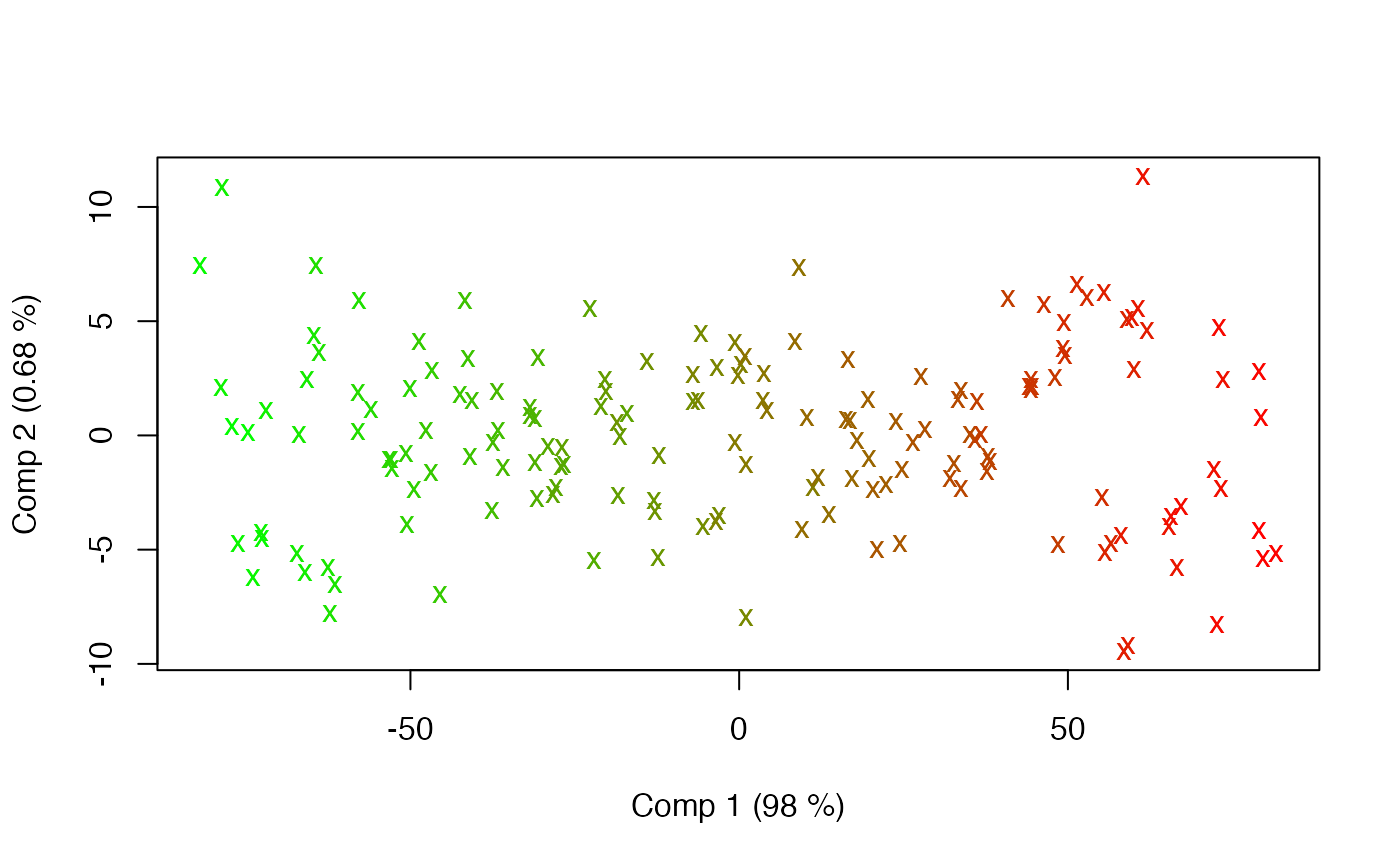
scoreplot(mod, factor=3, gr.col=rgb(eff/max(eff), 1-eff/max(eff),0), pch.scores="x")
# Numeric effects
candies$num <- eff <- 1:165
mod <- apca(assessment ~ candy + assessor + num, data=candies)
summary(mod)
#> Anova Principal Component Analysis fitted using 'lm' (Linear Model)
#> - SS type II, sum coding, restricted model, least squares estimation, SSQ method: qr_regression
#> Sum.Sq. Expl.var.(%)
#> candy 32438.46 72.30
#> assessor 1823.59 4.06
#> num 101.17 0.23
#> Residuals 9388.08 20.92
scoreplot(mod, factor=3, gr.col=rgb(eff/max(eff), 1-eff/max(eff),0), pch.scores="x")