Extraction of scores and loadings and adaptation of scoreplot,
loadingplot and biplot from package pls for sopls objects.
Usage
# S3 method for class 'sopls'
loadings(object, ncomp = "all", block = 1, y = FALSE, ...)

# S3 method for class 'sopls'
scores(object, ncomp = "all", block = 1, y = FALSE, ...)

# S3 method for class 'sopls'
scoreplot(
  object,
  comps = 1:2,
  ncomp = NULL,
  block = 1,
  labels,
  identify = FALSE,
  type = "p",
  xlab,
  ylab,
  ...
)

# S3 method for class 'sopls'
loadingplot(
  object,
  comps = 1:2,
  ncomp = NULL,
  block = 1,
  scatter = TRUE,
  labels,
  identify = FALSE,
  type,
  lty,
  lwd = NULL,
  pch,
  cex = NULL,
  col,
  legendpos,
  xlab,
  ylab,
  pretty.xlabels = TRUE,
  xlim,
  ...
)

# S3 method for class 'sopls'
corrplot(
  object,
  comps = 1:2,
  ncomp = NULL,
  block = 1,
  labels = TRUE,
  col = 1:5,
  plotx = TRUE,
  ploty = TRUE,
  ...
)

# S3 method for class 'sopls'
biplot(
  x,
  comps = 1:2,
  ncomp = "all",
  block = 1,
  which = c("x", "y", "scores", "loadings"),
  var.axes = FALSE,
  xlabs,
  ylabs,
  main,
  ...
)
Arguments
- object
soplsobject- ncomp
integervector giving components from all blocks beforeblock(see next argument).- block
integerindicating which block to extract components from.- y
logicalextract Y loadings/scores instead of X loadings/scores (default = FALSE).- ...
further arguments sent to the underlying plot function(s)
- comps
integervector giving components, within block, to plot (see Details regarding combination of blocks).- labels
characterindicating if "names" or "numbers" should be plot symbols (optional).- identify
logicalfor activatingidentifyto interactively identify points.- type
characterfor selecting type of plot to make. Defaults to "p" (points) for scatter plots and "l" (lines) for line plots.- xlab
charactertext for x labels.- ylab
charactertext for y labels.- scatter
logicalindicating if a scatterplot of loadings should be made (default = TRUE).- lty
Vector of line type specifications (see
parfor details).- lwd
numericvector of line width specifications.- pch
Vector of point specifications (see
pointsfor details).- cex
numericvector of plot size expansions (seeparfor details).- col
integervector of symbol/line colours (seeparfor details).- legendpos
characterindicating legend position (ifscatteris FALSE), e.g.legendpos = "topright".- pretty.xlabels
logicalindicating if xlabels should be more nicely plotted (default = TRUE).- xlim
numericvector of length two, with the x limits of the plot (optional).- plotx
locicalorinteger/character. Whether to plot the \(X\) correlation loadings, optionally which block(s). Defaults toTRUE.- ploty
logical. Whether to plot the \(Y\) correlation loadings. Defaults toTRUE.- x
soplsobject- which
characterfor selecting type of biplot ("x" = default, "y", "scores", "loadings").- var.axes
logicalindicating if second axes of a biplot should have arrows.- xlabs
charactervector for labelling first set of biplot points (optional).- ylabs
charactervector for labelling second set of biplot points (optional).- main
characterfor setting the main title of a plot.
Details
If comps is supplied as a list for scoreplot, it is assumed that its elements refer to each of the
blocks up to block number block. For instance comps = list(1, 0, 1:2) will select 1 component from the first
block, no components from the second block and the first two components from the last block. This must be
matched by ncomp, specifying how many components were selected before block number block.
See also
Overviews of available methods, multiblock, and methods organised by main structure: basic, unsupervised, asca, supervised and complex.
Common functions for computation and extraction of results are found in sopls_results.
#' @return The score and loading functions return scores and loadings, while plot functions have no return (except use of 'identify').
Examples
data(potato)
so <- sopls(Sensory ~ Chemical + Compression + NIRraw, data=potato, ncomp=c(5,5,5))

# Loadings
loadings(so, ncomp=c(3), block=2)[, 1:3]
#>          3,1,0       3,2,0        3,3,0
#> FW20  2.899592 -2.25518600 -1.181401337
#> BW20  3.253005 -0.34748421  0.211162557
#> ST20  3.232381  0.40110809 -0.042460853
#> SH20  2.450377 -3.89643043 -1.273002388
#> Mo20  1.471707  2.63506368 -0.950867682
#> Sl20  2.726383  0.26885897  0.002480118
#> FW750 3.159111 -0.21770583  0.551632015
#> BW750 2.892770  0.48171215  0.667057573
#> ST750 2.851268  0.01964503  0.173617022
#> SH750 3.370985 -1.53962601  1.348135225
#> Mo750 1.173309  1.92291778 -1.496492798
#> Sl750 2.539819  0.46410991 -0.071181501

# Scores
scores(so, block=1)[, 1:4]
#>           1,0,0       2,0,0        3,0,0       4,0,0
#> 1  -0.078379126 -0.15756558 -0.030150796 -0.08882899
#> 2   0.033599245  0.03345139 -0.264837392 -0.02082345
#> 3  -0.454087240 -0.50387774 -0.257625630  0.24822188
#> 4  -0.010144029  0.04409907  0.254739277  0.34206013
#> 5  -0.231320589  0.02813994  0.331647163 -0.15209020
#> 6  -0.100806072 -0.03203490  0.058511494 -0.07824489
#> 7   0.103759602  0.05587580  0.171495995  0.13245956
#> 8   0.142341829 -0.02952316  0.135315864  0.17766566
#> 9   0.160175421 -0.13395363  0.067732083 -0.34567441
#> 10  0.078862890 -0.20282246  0.065251294 -0.21205811
#> 11  0.200245777 -0.02882659  0.149667777 -0.08872396
#> 12  0.223602068 -0.07321286 -0.029748834 -0.22950703
#> 13  0.217320106 -0.26815383  0.096949900 -0.10070260
#> 14  0.142847549 -0.29951537  0.077252287  0.24996525
#> 15  0.213820293  0.17228886 -0.461863019 -0.11767172
#> 16  0.164964325  0.26005269 -0.323577542  0.10235857
#> 17  0.002967383  0.19480792 -0.246885356  0.19701818
#> 18  0.066258347  0.09356886 -0.228532411  0.20484080
#> 19  0.194213760 -0.01568159  0.132000297  0.14447620
#> 20  0.141301554 -0.07654188  0.049224760  0.26084474
#> 21 -0.129888279  0.04471652  0.038982799 -0.30565064
#> 22 -0.105636544  0.24576605 -0.030041538 -0.14535670
#> 23 -0.464479945 -0.11433433 -0.194275154 -0.06714686
#> 24 -0.082441922  0.22751259  0.233417343  0.13675311
#> 25 -0.325181587  0.44765983  0.208213841  0.07217114
#> 26 -0.103914818  0.08810440 -0.002864502 -0.31635566

# Default plot from first block
scoreplot(so)


# Second block with names
scoreplot(so, ncomp=c(3), block=2, labels="names")


# Scatterplot matrix
scoreplot(so, ncomp=c(3,2), block=3, comps=1:3)


# Combination of blocks (see Details)
scoreplot(so, ncomp=c(3,2), block=3, comps=list(1,0,1))


# Default plot from first block
loadingplot(so, scatter=TRUE)


# Second block with names
loadingplot(so, ncomp=c(3), block=2, labels="names", scatter=TRUE)


# Scatterplot matrix
loadingplot(so, ncomp=c(3,2), block=3, comps=1:3, scatter=TRUE)


# Correlation loadings
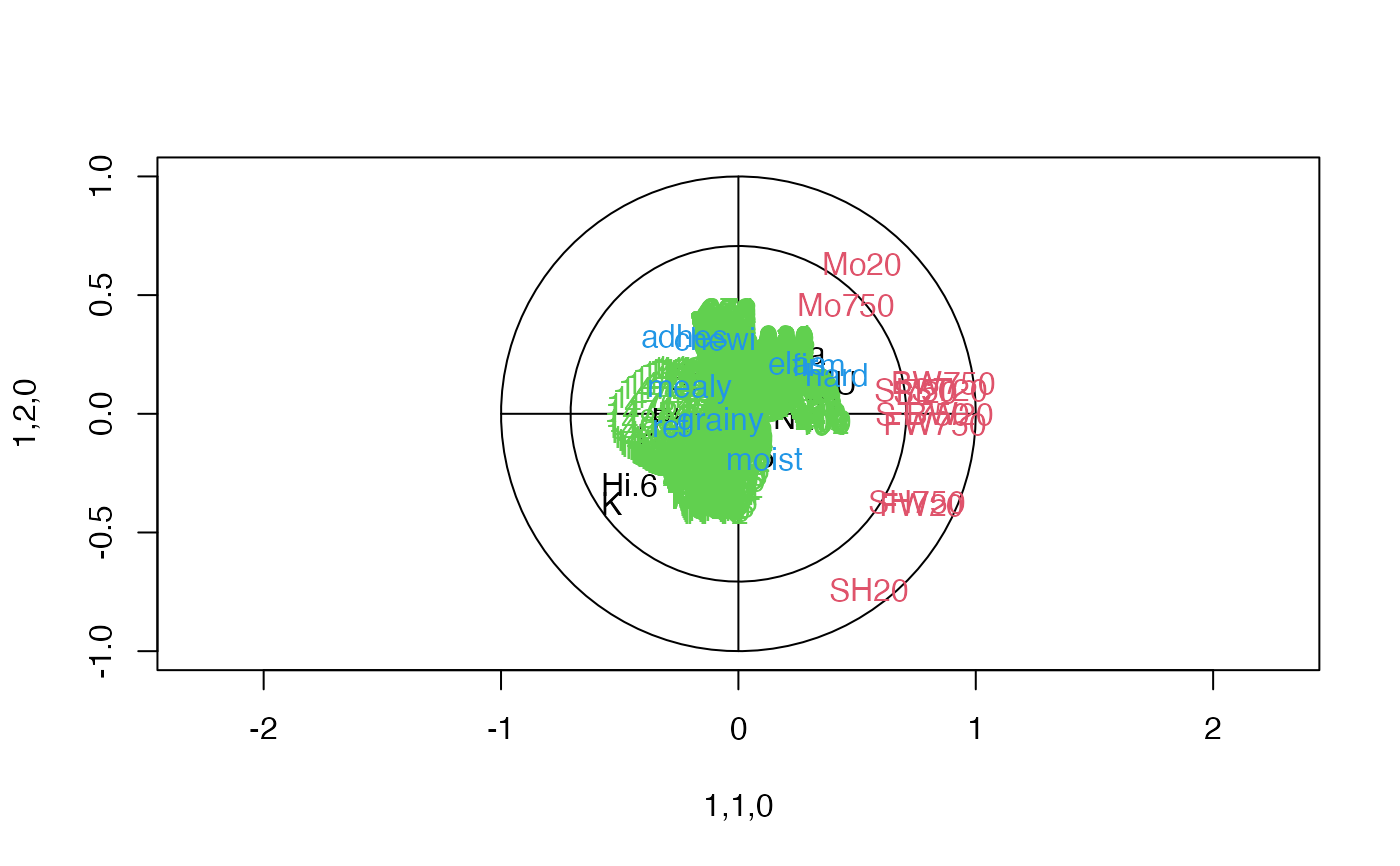
corrplot(so, block=2, ncomp=1)


# Default plot from first block
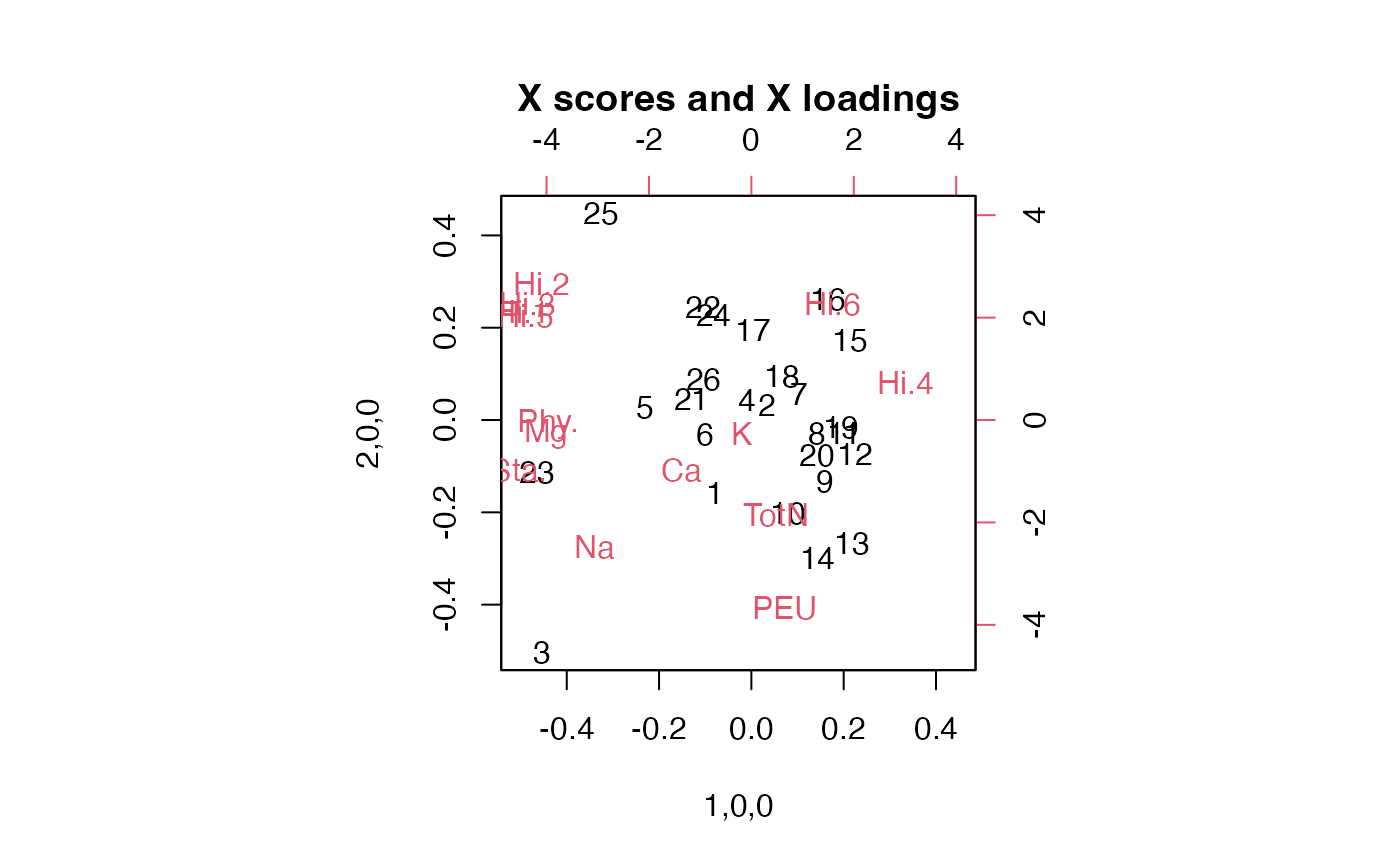
biplot(so)
