The (extended) ARIMA family of methods is too big to be properly explained in this course.
At NMBU, the course DAT320 goes deeper and explains the data generating processes.
An online book with videos: Forecasting: Principles and Practice.
We therefore skip (almost) directly to the regression models (inspired by phosgene89’s GitHub page, except for their errors) and their usage.
But first we introduce a dataset and the concepts of stationarity and autocorrelation.
Stationarity:
The distribution of the time series is independent of which part of the time series you look at.
Trends, seasonality (cycles of fixed width) and changes in variance lead to non-stationarity.
Differencing (first or second order discrete derivatives) can help.
Seasonal differencing means the difference is not between neighbours but higher lags.
If the data is not stationary, pre-processing or modelling of the specific deviations from stationarity is needed.
Wholesale price index (WPI) data
We will illustrate some concepts and models using the WPI data.
# Imports
import numpy as np
import pandas as pd
import statsmodels.api as sm
import matplotlib.pyplot as plt
import requests
from io import BytesIO

# Load Wholesale price index (WPI) data
wpi1 = requests.get('https://www.stata-press.com/data/r12/wpi1.dta').content
data = pd.read_stata(BytesIO(wpi1))
data.index = data.t
data['ln_wpi'] = np.log(data['wpi'])
data['D.ln_wpi'] = data['ln_wpi'].diff()
# Set the frequency to Quarterly Start, year ending October
data.index.freq="QS-OCT"
data.head()Autocorrelation
Autocorrelation is the correlation between a stationary timeseries and a lagged version of itself.
This is a measure of the time dependence in the series, i.e., lack of independence.
Can be used to indicate the appropriate lag in moving average (MA) models.
Partial autocorrelation is the autocorrelation when controlling for (regressed on) all intermediate time lags.
Can be used to indicate the appropriate lag in autogregressive (AR) models.
# Autocorrelation and partial autocorrelation plots (raw data)
fig, axes = plt.subplots(1, 2, figsize=(15,4))
fig = sm.graphics.tsa.plot_acf(data.iloc[1:]['wpi'], lags=40, ax=axes[0])
fig = sm.graphics.tsa.plot_pacf(data.iloc[1:]['wpi'], lags=40, ax=axes[1])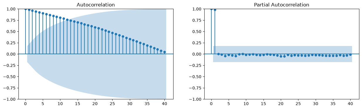
# Graph data
fig, axes = plt.subplots(1, 2, figsize=(12,3))

# Levels
axes[0].plot(data.index._mpl_repr(), data['wpi'], '-')
axes[0].set(title='US Wholesale Price Index')

# Log difference (attempting to improve stationarity)
axes[1].plot(data.index._mpl_repr(), data['D.ln_wpi'], '-')
axes[1].hlines(0, data.index[0], data.index[-1], 'r')
axes[1].set(title='US Wholesale Price Index - difference of logs');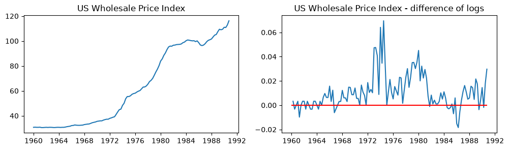
# Autocorrelation and partial autocorrelation plots
# after applying the logarithm and differencing
fig, axes = plt.subplots(1, 2, figsize=(12,3))
fig = sm.graphics.tsa.plot_acf(data.iloc[1:]['D.ln_wpi'], lags=40, ax=axes[0])
fig = sm.graphics.tsa.plot_pacf(data.iloc[1:]['D.ln_wpi'], lags=40, ax=axes[1])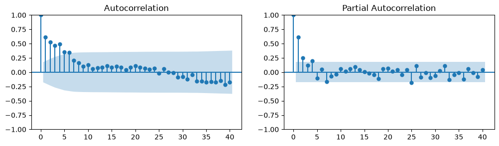
Autoregressive models in Python
Using the statsmodels package, the most complex model is the starting point.
Setting the various parameters of , we can obtain any of the below mentioned models.
SARIMAX(endog, exog=None, order=(1, 0, 0), seasonal_order=(0, 0, 0, 0), trend=None, ...)
For integer values of , all lags up to the integer are included. For more fine-grained control, lists can be applied, e.g., [1,0,1] includes lags 1 and 3, but not 2.
There are also various other parameters, e.g., a trend (none, constant, linear, quadratic, polynomial).
Lag operator
Back-shift time points, i.e., extracts the measurement time points before .
Also noted as in some litterature.
Combined with a vector of parameters , we define a polynomial function
This will enable compact notation of the SARIMAX models, exchanging sums with the polynomial function.
AR - autoregressive models
For a (single variable) timeseries given by , we can specify the model as:
i.e., the current time is a function of previous time points and a constant.
Here, is a constant, is the coefficient for the -th time lag and is the error.
This can be thought of as stacking subsets of a time series using a moving window and performing ordinary least squares on the resulting matrix/dataframe.
In practice, the fitting is performed using maximum likelihood, so performing ordinary regression will not give exactly the same results.
Using the lag operator, , we can redefine the above equation in the form of a polynomial function, (signs of coefficients will change) as:
# Fit an AR(1) model (badly specified due to non-stationarity)
mod = sm.tsa.statespace.SARIMAX(data['wpi'], trend='c', order=(1,0,0)) # trend='c' adds a constant
res = mod.fit(disp=False)
print(res.summary()) # AIC gives us a measure of fit for comparison
SARIMAX Results
==============================================================================
Dep. Variable: wpi No. Observations: 124
Model: SARIMAX(1, 0, 0) Log Likelihood -201.927
Date: Tue, 18 Aug 2026 AIC 409.855
Time: 14:20:32 BIC 418.316
Sample: 01-01-1960 HQIC 413.292
- 10-01-1990
Covariance Type: opg
==============================================================================
coef std err z P>|z| [0.025 0.975]
------------------------------------------------------------------------------
intercept 0.0293 0.343 0.086 0.932 -0.643 0.701
ar.L1 0.9996 0.005 213.302 0.000 0.990 1.009
sigma2 1.4355 0.143 10.008 0.000 1.154 1.717
===================================================================================
Ljung-Box (L1) (Q): 48.05 Jarque-Bera (JB): 20.69
Prob(Q): 0.00 Prob(JB): 0.00
Heteroskedasticity (H): 19.26 Skew: 0.90
Prob(H) (two-sided): 0.00 Kurtosis: 3.86
===================================================================================
Warnings:
[1] Covariance matrix calculated using the outer product of gradients (complex-step).
/Users/kristian/Documents/GitHub/IND320/.venv/lib/python3.12/site-packages/statsmodels/tsa/statespace/sarimax.py:966: UserWarning: Non-stationary starting autoregressive parameters found. Using zeros as starting parameters.
  warn('Non-stationary starting autoregressive parameters'
MA - moving average models
MA models are functions of previous errors, rather than previous measurements.
We can define an model as:
Here, is the number of time lags and is defined as above, but using the error terms and is with respect to the current model.
# Fit an MA(1) model (disregarding the obvious autocorrelation)
mod = sm.tsa.statespace.SARIMAX(data['wpi'], trend='c', order=(0,0,1))
res = mod.fit(disp=False)
print(res.summary()) # AIC gives us a measure of fit for comparison
SARIMAX Results
==============================================================================
Dep. Variable: wpi No. Observations: 124
Model: SARIMAX(0, 0, 1) Log Likelihood -516.522
Date: Tue, 18 Aug 2026 AIC 1039.044
Time: 14:20:33 BIC 1047.505
Sample: 01-01-1960 HQIC 1042.481
- 10-01-1990
Covariance Type: opg
==============================================================================
coef std err z P>|z| [0.025 0.975]
------------------------------------------------------------------------------
intercept 62.8671 3.033 20.727 0.000 56.922 68.812
ma.L1 0.9994 0.578 1.728 0.084 -0.134 2.133
sigma2 233.8562 132.640 1.763 0.078 -26.114 493.827
===================================================================================
Ljung-Box (L1) (Q): 114.21 Jarque-Bera (JB): 14.05
Prob(Q): 0.00 Prob(JB): 0.00
Heteroskedasticity (H): 1.55 Skew: 0.31
Prob(H) (two-sided): 0.17 Kurtosis: 1.47
===================================================================================
Warnings:
[1] Covariance matrix calculated using the outer product of gradients (complex-step).
/Users/kristian/Documents/GitHub/IND320/.venv/lib/python3.12/site-packages/statsmodels/tsa/statespace/sarimax.py:978: UserWarning: Non-invertible starting MA parameters found. Using zeros as starting parameters.
  warn('Non-invertible starting MA parameters found.'
ARMA - autoregressive moving average models
When we take the sum of and models of the same time series, we get models:
which can be reformulated to:
Again, is with respect to the current model, but shares name with the previous models.
This model is learning both from seeing previous samples and from how well these were predicted at previous time steps, thus it can tackle changes in the average.
# Fit an ARMA(1,1) model (badly specified due to non-stationarity)
mod = sm.tsa.statespace.SARIMAX(data['wpi'], trend='c', order=(1,0,1))
res = mod.fit(disp=False)
print(res.summary()) # AIC gives us a measure of fit for comparison
SARIMAX Results
==============================================================================
Dep. Variable: wpi No. Observations: 124
Model: SARIMAX(1, 0, 1) Log Likelihood -172.610
Date: Tue, 18 Aug 2026 AIC 353.221
Time: 14:20:33 BIC 364.502
Sample: 01-01-1960 HQIC 357.804
- 10-01-1990
Covariance Type: opg
==============================================================================
coef std err z P>|z| [0.025 0.975]
------------------------------------------------------------------------------
intercept 0.0438 0.427 0.103 0.918 -0.794 0.882
ar.L1 0.9994 0.006 172.091 0.000 0.988 1.011
ma.L1 0.5628 0.072 7.848 0.000 0.422 0.703
sigma2 0.8883 0.079 11.303 0.000 0.734 1.042
===================================================================================
Ljung-Box (L1) (Q): 0.80 Jarque-Bera (JB): 60.64
Prob(Q): 0.37 Prob(JB): 0.00
Heteroskedasticity (H): 15.38 Skew: 1.17
Prob(H) (two-sided): 0.00 Kurtosis: 5.51
===================================================================================
Warnings:
[1] Covariance matrix calculated using the outer product of gradients (complex-step).
/Users/kristian/Documents/GitHub/IND320/.venv/lib/python3.12/site-packages/statsmodels/tsa/statespace/sarimax.py:966: UserWarning: Non-stationary starting autoregressive parameters found. Using zeros as starting parameters.
  warn('Non-stationary starting autoregressive parameters'
ARIMA - autoregressive integrated moving average models
To help compensate for lack of stationarity, we add an integration operator, , defined as:
Here, and the degree of differensing is .
For instance with :
An model where is exchanged with would look like this:
The constant is often omitted and assumed absorbed by the integration. Only the time series is integrated, not the errors.
Reformulating this using the integration operator, we get an model:
This model has the properties of the ARMA model, but in addition does the differensing for us for stationarity.
The terms can be reorganised to get predictions on the original scale instead of predicting difference values.
# Fit an ARIMA(1,1,1) model
mod = sm.tsa.statespace.SARIMAX(data['wpi'], trend=None, order=(1,1,1))
res = mod.fit(disp=False)
print(res.summary()) # AIC gives us a measure of fit for comparison
SARIMAX Results
==============================================================================
Dep. Variable: wpi No. Observations: 124
Model: SARIMAX(1, 1, 1) Log Likelihood -137.247
Date: Tue, 18 Aug 2026 AIC 280.494
Time: 14:20:33 BIC 288.930
Sample: 01-01-1960 HQIC 283.920
- 10-01-1990
Covariance Type: opg
==============================================================================
coef std err z P>|z| [0.025 0.975]
------------------------------------------------------------------------------
ar.L1 0.9412 0.030 31.695 0.000 0.883 0.999
ma.L1 -0.4656 0.088 -5.314 0.000 -0.637 -0.294
sigma2 0.5398 0.054 10.071 0.000 0.435 0.645
===================================================================================
Ljung-Box (L1) (Q): 0.05 Jarque-Bera (JB): 9.12
Prob(Q): 0.82 Prob(JB): 0.01
Heteroskedasticity (H): 28.75 Skew: 0.07
Prob(H) (two-sided): 0.00 Kurtosis: 4.33
===================================================================================
Warnings:
[1] Covariance matrix calculated using the outer product of gradients (complex-step).
#### Fit an ARIMA(1,1,1) model
mod = sm.tsa.statespace.SARIMAX(data['wpi'], trend=None, order=(1,1,1))
res = mod.fit(disp=False)
print(res.summary()) # AIC gives us a measure of fit for comparison
SARIMAX Results
==============================================================================
Dep. Variable: wpi No. Observations: 124
Model: SARIMAX(1, 1, 1) Log Likelihood -137.247
Date: Tue, 18 Aug 2026 AIC 280.494
Time: 14:20:33 BIC 288.930
Sample: 01-01-1960 HQIC 283.920
- 10-01-1990
Covariance Type: opg
==============================================================================
coef std err z P>|z| [0.025 0.975]
------------------------------------------------------------------------------
ar.L1 0.9412 0.030 31.695 0.000 0.883 0.999
ma.L1 -0.4656 0.088 -5.314 0.000 -0.637 -0.294
sigma2 0.5398 0.054 10.071 0.000 0.435 0.645
===================================================================================
Ljung-Box (L1) (Q): 0.05 Jarque-Bera (JB): 9.12
Prob(Q): 0.82 Prob(JB): 0.01
Heteroskedasticity (H): 28.75 Skew: 0.07
Prob(H) (two-sided): 0.00 Kurtosis: 4.33
===================================================================================
Warnings:
[1] Covariance matrix calculated using the outer product of gradients (complex-step).
# Since the data are quarterly, we can add a seasonal component by including a fourth time lag to moving average
# Fit an ARIMA(1,1,[1,0,0,1]) model
mod = sm.tsa.statespace.SARIMAX(data['wpi'], trend=None, order=(1,1,[1,0,0,1]))
res = mod.fit(disp=False)
print(res.summary()) # AIC gives us a measure of fit for comparison
# What about a linear trend? (trend='t')
SARIMAX Results
=================================================================================
Dep. Variable: wpi No. Observations: 124
Model: SARIMAX(1, 1, [1, 4]) Log Likelihood -137.202
Date: Tue, 18 Aug 2026 AIC 282.404
Time: 14:20:33 BIC 293.653
Sample: 01-01-1960 HQIC 286.973
- 10-01-1990
Covariance Type: opg
==============================================================================
coef std err z P>|z| [0.025 0.975]
------------------------------------------------------------------------------
ar.L1 0.9313 0.041 22.884 0.000 0.852 1.011
ma.L1 -0.4540 0.093 -4.884 0.000 -0.636 -0.272
ma.L4 0.0433 0.082 0.526 0.599 -0.118 0.205
sigma2 0.5394 0.054 9.953 0.000 0.433 0.646
===================================================================================
Ljung-Box (L1) (Q): 0.04 Jarque-Bera (JB): 10.31
Prob(Q): 0.84 Prob(JB): 0.01
Heteroskedasticity (H): 29.04 Skew: 0.06
Prob(H) (two-sided): 0.00 Kurtosis: 4.41
===================================================================================
Warnings:
[1] Covariance matrix calculated using the outer product of gradients (complex-step).
SARIMA - seasonal autoregressive integrated moving average models
SARIMA shares some resemblance with the STL decomposition introduced previously.
For seasons of length , the seasonal part is obtained by applying an ARIMA model with lags, and , and integration time, , that are multiples of , i.e., if , the included time points would be and .
After the seasonal part has been removed, another is applied to which is equivalent to multiplying the two models together.
The model then becomes:
This model has the ability to combine experience from previous timepoints with seasonal trends.
Or if one sets the ARIMA parameters , , , one can have a pure seasonal model.
# Using SARIMA for seasonality instead of the fourth time lag to moving average.
# Fit a SARIMA(1,1,1)(1,1,1,4) model
mod = sm.tsa.statespace.SARIMAX(data['wpi'], trend=None, order=(1,1,1), seasonal_order=(1,1,1,4))
res = mod.fit(disp=False)
print(res.summary()) # AIC gives us a measure of fit for comparison (no improvement here)
SARIMAX Results
=========================================================================================
Dep. Variable: wpi No. Observations: 124
Model: SARIMAX(1, 1, 1)x(1, 1, 1, 4) Log Likelihood -135.889
Date: Tue, 18 Aug 2026 AIC 281.778
Time: 14:20:33 BIC 295.674
Sample: 01-01-1960 HQIC 287.421
- 10-01-1990
Covariance Type: opg
==============================================================================
coef std err z P>|z| [0.025 0.975]
------------------------------------------------------------------------------
ar.L1 0.8767 0.060 14.583 0.000 0.759 0.994
ma.L1 -0.3819 0.111 -3.453 0.001 -0.599 -0.165
ar.S.L4 0.0593 0.112 0.528 0.597 -0.161 0.279
ma.S.L4 -0.9978 2.221 -0.449 0.653 -5.351 3.356
sigma2 0.5187 1.127 0.460 0.645 -1.691 2.728
===================================================================================
Ljung-Box (L1) (Q): 0.07 Jarque-Bera (JB): 20.17
Prob(Q): 0.80 Prob(JB): 0.00
Heteroskedasticity (H): 29.33 Skew: -0.17
Prob(H) (two-sided): 0.00 Kurtosis: 4.99
===================================================================================
Warnings:
[1] Covariance matrix calculated using the outer product of gradients (complex-step).
Exogenous variables
As we showed in the previous chapter, it is possible to make a model purely on other variables measured at the same time, .
Including these variables into ARIMA and SARIMA, we get the ARIMAX and SARIMAX models.
In practice, we paste on an extra coefficient vector, , and variables, , to the models, here noted as sums of products :
:
:
The final model, thus includes autogression and moving averages, can perform differences, deals with seasonality and can leverage external variables from the same timepoint as the predictions.
# Read the FinalData sheet of the OilExchange.xlsx file using Pandas again
import pandas as pd
OilExchange = pd.read_excel('../../data/OilExchange.xlsx', sheet_name='FinalData')
OilExchange.index = OilExchange.Date
OilExchange.index.freq = "MS" # Set the frequency to Month Start
OilExchange.head()
/Users/kristian/Documents/GitHub/IND320/.venv/lib/python3.12/site-packages/openpyxl/worksheet/_reader.py:329: UserWarning: Unknown extension is not supported and will be removed
warn(msg)
# Fit a SARIMAX(1,1,1)(1,1,1,12) model with exogenous variables (closing our eyes, as we know little about the data)
mod = sm.tsa.statespace.SARIMAX(OilExchange['PerEURO'], exog=OilExchange.loc[:, OilExchange.columns[3:-6]], \
                                trend='c', order=(1,1,1), seasonal_order=(1,1,1,12))
res = mod.fit(disp=False)
print(res.summary()) # AIC gives us a measure of fit for comparison (no improvement here)
SARIMAX Results
==========================================================================================
Dep. Variable: PerEURO No. Observations: 179
Model: SARIMAX(1, 1, 1)x(1, 1, 1, 12) Log Likelihood 103.848
Date: Tue, 18 Aug 2026 AIC -157.695
Time: 14:20:35 BIC -79.896
Sample: 01-01-2000 HQIC -126.116
- 11-01-2014
Covariance Type: opg
======================================================================================
coef std err z P>|z| [0.025 0.975]
--------------------------------------------------------------------------------------
intercept 0.0011 0.018 0.061 0.951 -0.034 0.037
KeyIntRate -0.2262 0.279 -0.810 0.418 -0.773 0.321
LoanIntRate -0.0130 0.254 -0.051 0.959 -0.511 0.485
EuroIntRate 0.2143 0.107 2.009 0.045 0.005 0.423
CPI -0.0051 0.028 -0.180 0.857 -0.061 0.050
OilSpotPrice -0.0043 0.001 -3.124 0.002 -0.007 -0.002
ImpOldShip -0.0144 0.021 -0.684 0.494 -0.056 0.027
ImpNewShip -0.0144 0.021 -0.685 0.493 -0.056 0.027
ImpOilPlat -0.0144 0.021 -0.686 0.493 -0.056 0.027
ImpExShipOilPlat -0.0005 0.023 -0.021 0.983 -0.045 0.044
ExpCrdOil -0.0026 0.015 -0.172 0.863 -0.032 0.027
ExpNatGas -0.0026 0.015 -0.171 0.864 -0.032 0.027
ExpCond -0.0026 0.015 -0.172 0.864 -0.032 0.027
ExpOldShip 0.0144 0.021 0.684 0.494 -0.027 0.056
ExpNewShip 0.0144 0.021 0.685 0.493 -0.027 0.056
ExpOilPlat 0.0144 0.021 0.686 0.492 -0.027 0.056
ExpExShipOilPlat 0.0005 0.023 0.021 0.983 -0.044 0.045
TrBal -0.0144 0.021 -0.685 0.493 -0.056 0.027
TrBalExShipOilPlat 0.0165 0.019 0.852 0.394 -0.022 0.055
TrBalMland -0.0026 0.015 -0.172 0.863 -0.032 0.027
ar.L1 -0.7115 0.275 -2.587 0.010 -1.251 -0.172
ma.L1 0.8770 0.186 4.716 0.000 0.513 1.241
ar.S.L12 -0.2670 0.218 -1.223 0.221 -0.695 0.161
ma.S.L12 -0.4389 0.228 -1.926 0.054 -0.885 0.008
sigma2 0.0225 0.004 5.584 0.000 0.015 0.030
===================================================================================
Ljung-Box (L1) (Q): 0.59 Jarque-Bera (JB): 1.54
Prob(Q): 0.44 Prob(JB): 0.46
Heteroskedasticity (H): 0.91 Skew: 0.11
Prob(H) (two-sided): 0.72 Kurtosis: 3.41
===================================================================================
Warnings:
[1] Covariance matrix calculated using the outer product of gradients (complex-step).
/Users/kristian/Documents/GitHub/IND320/.venv/lib/python3.12/site-packages/statsmodels/base/model.py:607: ConvergenceWarning: Maximum Likelihood optimization failed to converge. Check mle_retvals
  warnings.warn("Maximum Likelihood optimization failed to "
Exercise
Play with the OilExchange data.
See if you can improve the fit of the model by adjusting lags and removing the least significant terms in the model.
Interpretation of Model Diagnostic Tests
Ljung-Box (L1) (Q)
Purpose: Tests for autocorrelation in the residuals.
Null hypothesis (H₀): The residuals are independently distributed (no autocorrelation up to lag L1).
Result:
Q: test statistic
Prob(Q): >0.05 is good
Jarque-Bera (JB)
Purpose: Tests whether the residuals are normally distributed (based on skewness and kurtosis).
Null hypothesis (H₀): The residuals are normally distributed.
Result:
JB: test statistic
Prob(JB): >0.05 is good
Heteroskedasticity (H)
Purpose: Tests whether the residuals have constant variance (homoskedasticity).
Null hypothesis (H₀): The residuals have constant variance.
Result:
H: test statistic
Prob(H): >0.05 is good
Skew and Kurtosis
Skew: Measures asymmetry of the residuals. 0 means symmetric; positive means right-skewed.
Kurtosis: Measures “tailedness” of the residuals. 3 is normal; higher means heavier tails.
In practice:
Independence and constant variance are more important for forecasting than perfect normality.
Non-normality is common in real-world time series models.
SARIMAX prediction
One-step-ahead prediction uses the estimated parameters and samples within the lags of the model to predict the next time point.
This means that the predictions will stay relatively close to the true values, never predicting more than one step away from the truth.
Dynamic prediction predicts one step as above, then uses predicted values as input instead of true values.
This means the predictions can deviate from the truth over time.
# Refit the model on the training set (up to 2013-01-01) to estimate the parameters
mod = sm.tsa.statespace.SARIMAX(OilExchange['PerEURO'].loc[:'2013-01-01'], \
                                OilExchange.loc[:, OilExchange.columns[3:-4]].loc[:'2013-01-01'], \
    trend='c', order=(1,1,1), seasonal_order=(1,1,1,12))
res = mod.fit(disp=False)
/Users/kristian/Documents/GitHub/IND320/.venv/lib/python3.12/site-packages/statsmodels/tsa/statespace/sarimax.py:966: UserWarning: Non-stationary starting autoregressive parameters found. Using zeros as starting parameters.
warn('Non-stationary starting autoregressive parameters'
/Users/kristian/Documents/GitHub/IND320/.venv/lib/python3.12/site-packages/statsmodels/tsa/statespace/sarimax.py:978: UserWarning: Non-invertible starting MA parameters found. Using zeros as starting parameters.
warn('Non-invertible starting MA parameters found.'
/Users/kristian/Documents/GitHub/IND320/.venv/lib/python3.12/site-packages/statsmodels/base/model.py:607: ConvergenceWarning: Maximum Likelihood optimization failed to converge. Check mle_retvals
  warnings.warn("Maximum Likelihood optimization failed to "
# Get predictions for the whole dataset
mod = sm.tsa.statespace.SARIMAX(OilExchange['PerEURO'], OilExchange.loc[:, OilExchange.columns[3:-4]], \
    trend='c', order=(1,1,1), seasonal_order=(1,1,1,12))

res = mod.filter(res.params) # One-step-ahead predictions using parameters from previous fit
# In-sample one-step-ahead prediction wrapper function
predict = res.get_prediction()
predict_ci = predict.conf_int()# Dynamic predictions starting from 2013-01-01
predict_dy = res.get_prediction(dynamic='2013-01-01')
predict_dy_ci = predict_dy.conf_int()# Compare the one-step-ahead predictions to the dynamic predictions
fig, ax = plt.subplots(figsize=(9,4))
npre = 4
ax.set(title='Exchange rate', xlabel='Date', ylabel='Per EURO')
# Plot data points
OilExchange.loc['2012-01-01':, 'PerEURO'].plot(ax=ax, style='o', label='Observed')
# Plot predictions
predict.predicted_mean.loc['2012-01-01':].plot(ax=ax, style='r--', label='One-step-ahead forecast')
ci = predict_ci.loc['2012-01-01':]
ax.fill_between(ci.index, ci.iloc[:,0], ci.iloc[:,1], color='r', alpha=0.1)
predict_dy.predicted_mean.loc['2012-01-01':].plot(ax=ax, style='g', label='Dynamic forecast (2013)')
ci = predict_dy_ci.loc['2012-01-01':]
ax.fill_between(ci.index, ci.iloc[:,0], ci.iloc[:,1], color='g', alpha=0.1)
legend = ax.legend(loc='lower right')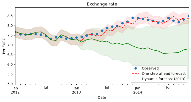
Questercise
Does the model made in the previous exercise improve the predictions as visualized above?