Machine Learning approach - Data to Decision

Time series prediction, or forecasting, can be very similar to modelling and prediction with tabular data.
- A set of input variables, usually a single output variable.
- Ordinary machine learning methods can be applied.
The inclusion of time can be done by adding one or more delayed variables, possibly including the response.

Validation¶

As soon as time is part of a model, extra care needs to be taken in validation.
Cross-validation*, training-validation-test splits are still relevant.
However, training, validation and test sets need to follow time chronologically and cannot overlap.
Instead of traditional cross-validation, one can perform backtesting with a sliding or expanding window:

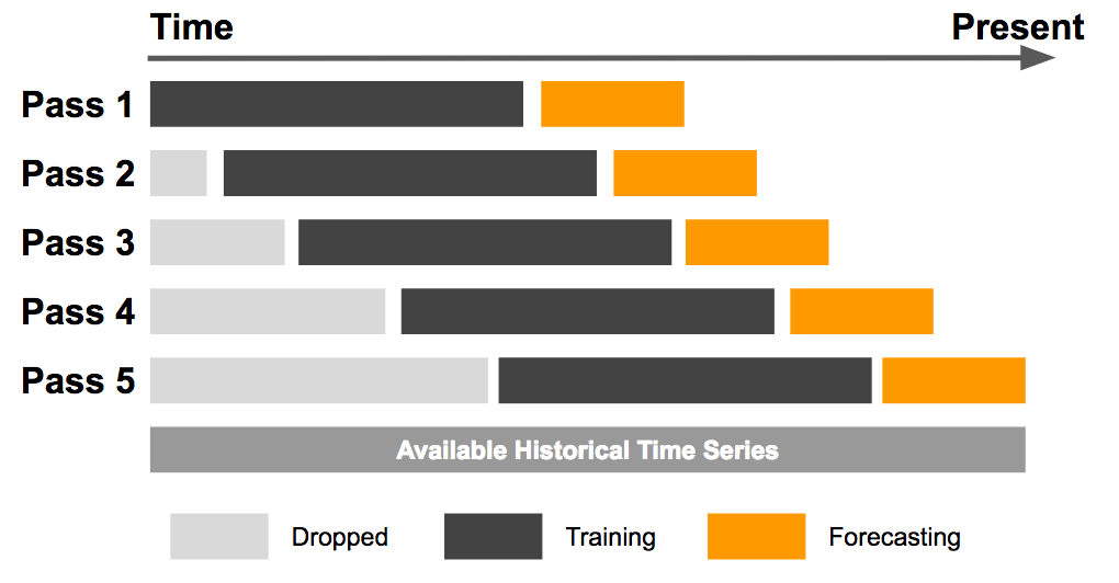
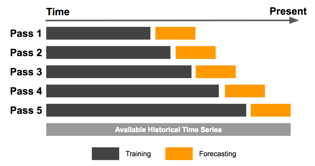
Figures from Roy Yang’s bloggpost on uber.com

Shipping, oil, interest rates and exchange rates¶

These data are public data from the Norwegian Bank, SSB, Eurostat and U.S. Energy Information Administration for the period 2000-2014 (monthly).
The data are available at ResearchGate and were part of a Master thesis by Raju Rimal.

# Read the FinalData sheet of the OilExchange.xlsx file using Pandas
import pandas as pd
# You may get a warning here, because the file contains pasted grahics
OilExchange = pd.read_excel('../../data/OilExchange.xlsx', sheet_name='FinalData') 
OilExchange.head()

/Users/kristian/Documents/GitHub/IND320/.venv/lib/python3.12/site-packages/openpyxl/worksheet/_reader.py:329: UserWarning: Unknown extension is not supported and will be removed
  warn(msg)

OilExchange.columns

Index(['Date', 'PerEURO', 'PerUSD', 'KeyIntRate', 'LoanIntRate', 'EuroIntRate',
       'CPI', 'OilSpotPrice', 'ImpOldShip', 'ImpNewShip', 'ImpOilPlat',
       'ImpExShipOilPlat', 'ExpCrdOil', 'ExpNatGas', 'ExpCond', 'ExpOldShip',
       'ExpNewShip', 'ExpOilPlat', 'ExpExShipOilPlat', 'TrBal',
       'TrBalExShipOilPlat', 'TrBalMland', 'ly.var', 'l2y.var', 'l.CPI',
       'ExcChange', 'Testrain', 'season'],
      dtype='str')

# Read the FinalCodeBook sheet of the OilExchange.xlsx file using Pandas
Explanations = pd.read_excel('../../data/OilExchange.xlsx', sheet_name='FinalCodeBook')
Explanations[['Variables','Label']]

/Users/kristian/Documents/GitHub/IND320/.venv/lib/python3.12/site-packages/openpyxl/worksheet/_reader.py:329: UserWarning: Unknown extension is not supported and will be removed
  warn(msg)

Modelling without time¶

For starters, let us ignore time and build a simple prediction model for the exchange rate.
We will use scikit-learn’s Pipeline to combine standardisation (scaling) and linear regression and cross_val_predict to perform random K-fold cross-validation.

# Import Pipeline, StandardScaler, and LinearRegression from their respective modules in sklearn
from sklearn.pipeline import Pipeline
from sklearn.preprocessing import StandardScaler
from sklearn.linear_model import LinearRegression

# Create a pipeline that scales the data and performs linear regression
pipe = Pipeline([('scaler', StandardScaler()), ('reg', LinearRegression())])

# Fit the pipeline with PerEURO as response and variables 3:-6 as predictors for the samples having True in the Testrain column
OilExchange_train = OilExchange.loc[OilExchange.Testrain==True,:].copy()
OilExchange_test = OilExchange.loc[OilExchange.Testrain==False,:].copy()
pipe.fit(OilExchange_train.loc[:, OilExchange_train.columns[3:-6]], \
         OilExchange_train.loc[:, 'PerEURO'])

# Predict the corresponding data for Testrain = False
PerEURO_pred = pipe.predict(OilExchange_test.loc[:, OilExchange.columns[3:-6]])

# Plot the predicted values against the actual values
import matplotlib.pyplot as plt
plt.scatter(OilExchange_test.loc[:, 'PerEURO'], PerEURO_pred)
plt.xlabel('Actual PerEURO')
plt.ylabel('Predicted PerEURO')
plt.title('Test data predictions')
plt.show()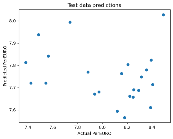

# R2 for the test data
from sklearn.metrics import r2_score
r2_score(OilExchange_test.loc[:, 'PerEURO'], PerEURO_pred)

-0.9790095192601644

# Perform k-fold cross-validation with k=10
from sklearn.model_selection import cross_val_predict # NOTE: Not for time series!
PerEURO_cv = cross_val_predict(pipe, OilExchange_train.loc[:, OilExchange.columns[3:-6]], \
                               OilExchange_train.loc[:, 'PerEURO'], cv=10)

# Compute R^2 for PerEURO_cv
r2_cv = r2_score(OilExchange_train.loc[:, 'PerEURO'], PerEURO_cv)
print("Cross-validated R2: {:.3f}".format(r2_cv))

Cross-validated R2: -0.317

Backtesting¶

scikit-learn has a TimeSeriesSplit which creates segments for backtesting.
- Expanding window is the default.
- Sliding window can be applied by setting the right combination of parameters.
We will use scikit-learn’s cross_validate to perform the cross-validation based on the backtesting segments (cross_val_predict assumes that all observations will be test data at some point).

# Backtesting using scikit-learn
import numpy as np
from sklearn.model_selection import TimeSeriesSplit

# Some data
X = np.array([[1, 2], [3, 4], [1, 2], [3, 4], [1, 2], [3, 4]])
y = np.array([1, 2, 3, 4, 5, 6])

# Create time series cross-validation object with expanding window
tscv_expand = TimeSeriesSplit()
print(tscv_expand)
for i, (train_index, test_index) in enumerate(tscv_expand.split(X)):
    print(f"Fold {i}:")
    print(f"  Train: index={train_index}")
    print(f"  Test:  index={test_index}")

TimeSeriesSplit(gap=0, max_train_size=None, n_splits=5, test_size=None)
Fold 0:
  Train: index=[0]
  Test:  index=[1]
Fold 1:
  Train: index=[0 1]
  Test:  index=[2]
Fold 2:
  Train: index=[0 1 2]
  Test:  index=[3]
Fold 3:
  Train: index=[0 1 2 3]
  Test:  index=[4]
Fold 4:
  Train: index=[0 1 2 3 4]
  Test:  index=[5]

# Backtesting with sliding window
tscv_slide = TimeSeriesSplit(max_train_size=3, n_splits=3)
print(tscv_slide)
for i, (train_index, test_index) in enumerate(tscv_slide.split(X)):
    print(f"Fold {i}:")
    print(f"  Train: index={train_index}")
    print(f"  Test:  index={test_index}")

TimeSeriesSplit(gap=0, max_train_size=3, n_splits=3, test_size=None)
Fold 0:
  Train: index=[0 1 2]
  Test:  index=[3]
Fold 1:
  Train: index=[1 2 3]
  Test:  index=[4]
Fold 2:
  Train: index=[2 3 4]
  Test:  index=[5]

# Backtesting with expanding window in the OilExchange data
tscv_expand = TimeSeriesSplit(n_splits=10)

# The segments
max_train = []
for i, (train_index, test_index) in enumerate(tscv_expand.split(OilExchange_train.loc[:, 'PerEURO'])):
    print(f"Fold {i}:")
    print(f"  Train: index={train_index}")
    max_train.append(max(train_index))
    print(f"  Test:  index={test_index}")

Fold 0:
  Train: index=[ 0  1  2  3  4  5  6  7  8  9 10 11 12 13 14 15]
  Test:  index=[16 17 18 19 20 21 22 23 24 25 26 27 28 29]
Fold 1:
  Train: index=[ 0  1  2  3  4  5  6  7  8  9 10 11 12 13 14 15 16 17 18 19 20 21 22 23
 24 25 26 27 28 29]
  Test:  index=[30 31 32 33 34 35 36 37 38 39 40 41 42 43]
Fold 2:
  Train: index=[ 0  1  2  3  4  5  6  7  8  9 10 11 12 13 14 15 16 17 18 19 20 21 22 23
 24 25 26 27 28 29 30 31 32 33 34 35 36 37 38 39 40 41 42 43]
  Test:  index=[44 45 46 47 48 49 50 51 52 53 54 55 56 57]
Fold 3:
  Train: index=[ 0  1  2  3  4  5  6  7  8  9 10 11 12 13 14 15 16 17 18 19 20 21 22 23
 24 25 26 27 28 29 30 31 32 33 34 35 36 37 38 39 40 41 42 43 44 45 46 47
 48 49 50 51 52 53 54 55 56 57]
  Test:  index=[58 59 60 61 62 63 64 65 66 67 68 69 70 71]
Fold 4:
  Train: index=[ 0  1  2  3  4  5  6  7  8  9 10 11 12 13 14 15 16 17 18 19 20 21 22 23
 24 25 26 27 28 29 30 31 32 33 34 35 36 37 38 39 40 41 42 43 44 45 46 47
 48 49 50 51 52 53 54 55 56 57 58 59 60 61 62 63 64 65 66 67 68 69 70 71]
  Test:  index=[72 73 74 75 76 77 78 79 80 81 82 83 84 85]
Fold 5:
  Train: index=[ 0  1  2  3  4  5  6  7  8  9 10 11 12 13 14 15 16 17 18 19 20 21 22 23
 24 25 26 27 28 29 30 31 32 33 34 35 36 37 38 39 40 41 42 43 44 45 46 47
 48 49 50 51 52 53 54 55 56 57 58 59 60 61 62 63 64 65 66 67 68 69 70 71
 72 73 74 75 76 77 78 79 80 81 82 83 84 85]
  Test:  index=[86 87 88 89 90 91 92 93 94 95 96 97 98 99]
Fold 6:
  Train: index=[ 0  1  2  3  4  5  6  7  8  9 10 11 12 13 14 15 16 17 18 19 20 21 22 23
 24 25 26 27 28 29 30 31 32 33 34 35 36 37 38 39 40 41 42 43 44 45 46 47
 48 49 50 51 52 53 54 55 56 57 58 59 60 61 62 63 64 65 66 67 68 69 70 71
 72 73 74 75 76 77 78 79 80 81 82 83 84 85 86 87 88 89 90 91 92 93 94 95
 96 97 98 99]
  Test:  index=[100 101 102 103 104 105 106 107 108 109 110 111 112 113]
Fold 7:
  Train: index=[  0   1   2   3   4   5   6   7   8   9  10  11  12  13  14  15  16  17
  18  19  20  21  22  23  24  25  26  27  28  29  30  31  32  33  34  35
  36  37  38  39  40  41  42  43  44  45  46  47  48  49  50  51  52  53
  54  55  56  57  58  59  60  61  62  63  64  65  66  67  68  69  70  71
  72  73  74  75  76  77  78  79  80  81  82  83  84  85  86  87  88  89
  90  91  92  93  94  95  96  97  98  99 100 101 102 103 104 105 106 107
 108 109 110 111 112 113]
  Test:  index=[114 115 116 117 118 119 120 121 122 123 124 125 126 127]
Fold 8:
  Train: index=[  0   1   2   3   4   5   6   7   8   9  10  11  12  13  14  15  16  17
  18  19  20  21  22  23  24  25  26  27  28  29  30  31  32  33  34  35
  36  37  38  39  40  41  42  43  44  45  46  47  48  49  50  51  52  53
  54  55  56  57  58  59  60  61  62  63  64  65  66  67  68  69  70  71
  72  73  74  75  76  77  78  79  80  81  82  83  84  85  86  87  88  89
  90  91  92  93  94  95  96  97  98  99 100 101 102 103 104 105 106 107
 108 109 110 111 112 113 114 115 116 117 118 119 120 121 122 123 124 125
 126 127]
  Test:  index=[128 129 130 131 132 133 134 135 136 137 138 139 140 141]
Fold 9:
  Train: index=[  0   1   2   3   4   5   6   7   8   9  10  11  12  13  14  15  16  17
  18  19  20  21  22  23  24  25  26  27  28  29  30  31  32  33  34  35
  36  37  38  39  40  41  42  43  44  45  46  47  48  49  50  51  52  53
  54  55  56  57  58  59  60  61  62  63  64  65  66  67  68  69  70  71
  72  73  74  75  76  77  78  79  80  81  82  83  84  85  86  87  88  89
  90  91  92  93  94  95  96  97  98  99 100 101 102 103 104 105 106 107
 108 109 110 111 112 113 114 115 116 117 118 119 120 121 122 123 124 125
 126 127 128 129 130 131 132 133 134 135 136 137 138 139 140 141]
  Test:  index=[142 143 144 145 146 147 148 149 150 151 152 153 154 155]

# Backtesting using expanding window with data
from sklearn.model_selection import cross_validate
scores = cross_validate(pipe, OilExchange_train.loc[:, OilExchange_train.columns[3:-6]], \
                                 OilExchange_train.loc[:, 'PerEURO'], cv=tscv_expand, \
                                    scoring='r2', return_train_score=True)
scores

{'fit_time': array([0.0034461 , 0.00206327, 0.00166082, 0.0033648 , 0.00181198,
        0.00175905, 0.00186896, 0.00169396, 0.00247335, 0.00195909]),
 'score_time': array([0.00135779, 0.00083685, 0.00075603, 0.00183201, 0.00081897,
        0.00078726, 0.00079513, 0.00079513, 0.00439095, 0.00083303]),
 'test_score': array([-2.58120320e+03, -4.49066361e+00, -7.37304826e+00,  1.20667734e-01,
        -5.47564370e+00, -1.91343710e+01, -1.62104880e+00, -2.82911176e-02,
        -3.42287951e+00, -1.33079128e+01]),
 'train_score': array([1.        , 0.95668789, 0.92040214, 0.85950793, 0.84569018,
        0.78860664, 0.69881999, 0.68809706, 0.65576638, 0.64771763])}

# Plot the backtesting results for train and test data, and under it ad the original data (PerEURO) as a subplot
plt.subplot(2,1,1)
plt.plot(scores['train_score'], label='Train')
plt.plot(scores['test_score'], label='Test')
plt.xlabel('Fold')
plt.ylabel('R$^2$')
plt.title('Backtesting results')
plt.axhline(0, color='gray', linestyle='--')
plt.ylim(-1.6,1.1)
plt.legend()
plt.subplot(2,1,2)
plt.plot(OilExchange_train.loc[:, 'PerEURO'])
for i in range(10):
    plt.axvline(x=max_train[i], color='gray', linestyle='--')
plt.xlabel('Time')
plt.ylabel('PerEURO')
plt.tight_layout()
plt.show()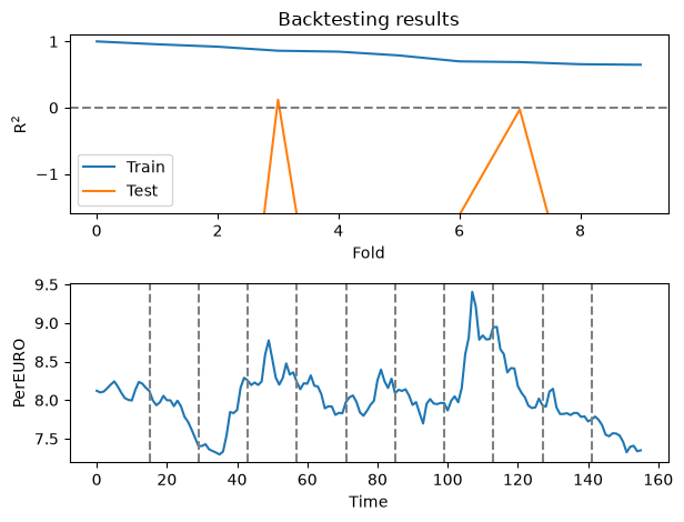

Question: Does the behaviour make sense with regard to what is included in and predicted from the model?

# Backtesting with sliding window in the OilExchange data
tscv_slide = TimeSeriesSplit(max_train_size=45, n_splits=10)

# The segments
max_train = []
for i, (train_index, test_index) in enumerate(tscv_slide.split(OilExchange_train.loc[:, 'PerEURO'])):
    print(f"Fold {i}:")
    print(f"  Train: index={train_index}")
    max_train.append(max(train_index))
    print(f"  Test:  index={test_index}")

Fold 0:
  Train: index=[ 0  1  2  3  4  5  6  7  8  9 10 11 12 13 14 15]
  Test:  index=[16 17 18 19 20 21 22 23 24 25 26 27 28 29]
Fold 1:
  Train: index=[ 0  1  2  3  4  5  6  7  8  9 10 11 12 13 14 15 16 17 18 19 20 21 22 23
 24 25 26 27 28 29]
  Test:  index=[30 31 32 33 34 35 36 37 38 39 40 41 42 43]
Fold 2:
  Train: index=[ 0  1  2  3  4  5  6  7  8  9 10 11 12 13 14 15 16 17 18 19 20 21 22 23
 24 25 26 27 28 29 30 31 32 33 34 35 36 37 38 39 40 41 42 43]
  Test:  index=[44 45 46 47 48 49 50 51 52 53 54 55 56 57]
Fold 3:
  Train: index=[13 14 15 16 17 18 19 20 21 22 23 24 25 26 27 28 29 30 31 32 33 34 35 36
 37 38 39 40 41 42 43 44 45 46 47 48 49 50 51 52 53 54 55 56 57]
  Test:  index=[58 59 60 61 62 63 64 65 66 67 68 69 70 71]
Fold 4:
  Train: index=[27 28 29 30 31 32 33 34 35 36 37 38 39 40 41 42 43 44 45 46 47 48 49 50
 51 52 53 54 55 56 57 58 59 60 61 62 63 64 65 66 67 68 69 70 71]
  Test:  index=[72 73 74 75 76 77 78 79 80 81 82 83 84 85]
Fold 5:
  Train: index=[41 42 43 44 45 46 47 48 49 50 51 52 53 54 55 56 57 58 59 60 61 62 63 64
 65 66 67 68 69 70 71 72 73 74 75 76 77 78 79 80 81 82 83 84 85]
  Test:  index=[86 87 88 89 90 91 92 93 94 95 96 97 98 99]
Fold 6:
  Train: index=[55 56 57 58 59 60 61 62 63 64 65 66 67 68 69 70 71 72 73 74 75 76 77 78
 79 80 81 82 83 84 85 86 87 88 89 90 91 92 93 94 95 96 97 98 99]
  Test:  index=[100 101 102 103 104 105 106 107 108 109 110 111 112 113]
Fold 7:
  Train: index=[ 69  70  71  72  73  74  75  76  77  78  79  80  81  82  83  84  85  86
  87  88  89  90  91  92  93  94  95  96  97  98  99 100 101 102 103 104
 105 106 107 108 109 110 111 112 113]
  Test:  index=[114 115 116 117 118 119 120 121 122 123 124 125 126 127]
Fold 8:
  Train: index=[ 83  84  85  86  87  88  89  90  91  92  93  94  95  96  97  98  99 100
 101 102 103 104 105 106 107 108 109 110 111 112 113 114 115 116 117 118
 119 120 121 122 123 124 125 126 127]
  Test:  index=[128 129 130 131 132 133 134 135 136 137 138 139 140 141]
Fold 9:
  Train: index=[ 97  98  99 100 101 102 103 104 105 106 107 108 109 110 111 112 113 114
 115 116 117 118 119 120 121 122 123 124 125 126 127 128 129 130 131 132
 133 134 135 136 137 138 139 140 141]
  Test:  index=[142 143 144 145 146 147 148 149 150 151 152 153 154 155]

# Backtesting using sliding window with data
from sklearn.model_selection import cross_validate
scores = cross_validate(pipe, OilExchange_train.loc[:, OilExchange_train.columns[3:-4]], \
                                 OilExchange_train.loc[:, 'PerEURO'], cv=tscv_slide, \
                                    scoring='r2', return_train_score=True)
scores

{'fit_time': array([0.01077986, 0.00419188, 0.00206995, 0.00275826, 0.00767589,
        0.00313282, 0.00351477, 0.00156379, 0.00197911, 0.00196409]),
 'score_time': array([0.00166607, 0.00104213, 0.00108099, 0.00119996, 0.00208116,
        0.00100899, 0.00082731, 0.00070882, 0.00081372, 0.00159621]),
 'test_score': array([-2.69048314e+03, -1.24210053e+00, -1.33007709e+00,  6.61087698e-01,
        -8.82686693e+00, -3.59907774e+02,  5.20015261e-01, -2.78711930e+00,
        -7.94540852e+04,  4.04120248e-01]),
 'train_score': array([1.        , 0.99034575, 0.95542869, 0.94013477, 0.95627895,
        0.8961227 , 0.75351647, 0.96129276, 0.93446863, 0.94984244])}

# Plot the backtesting results for train and test data, and under it ad the original data (PerEURO) as a subplot
plt.subplot(2,1,1)
plt.plot(scores['train_score'], label='Train')
plt.plot(scores['test_score'], label='Test')
plt.xlabel('Fold')
plt.ylabel('R$^2$')
plt.title('Backtesting results')
plt.axhline(0, color='gray', linestyle='--')
plt.ylim(-1.6,1.1)
plt.legend()
plt.subplot(2,1,2)
plt.plot(OilExchange_train.loc[:, 'PerEURO'])
for i in range(10):
    plt.axvline(x=max_train[i], color='gray', linestyle='--')
plt.xlabel('Time')
plt.ylabel('PerEURO')
plt.tight_layout()
plt.show()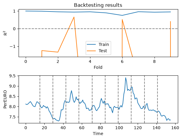

Question: Again; does the behaviour make sense with regard to what is included in and predicted from the model?

Exercise¶

Repeat the PerEuro predictions, but exchange LinearRegression with scikit-learns’s PLSRegression.
Check if the number of components in the PLS model has an effect on the explained variance ( $\text{R}^2$ ), either manually or using a GridSearchCV.

Including the response variable in the predictors¶

As long as the training and test sets are not overlapping, we can include the response as a predictor.
Adding the response lagged can be done as a single variable or several variables (i.e., several different lags).
We will later look at ARIMA-type models where time lag is the main mechanism for modelling.

# Add the Per Euro column to the OilExchange data but shifted 1 timepoint backwards (and backfill last value)
OilExchange_train['PerEURO_lag1'] = OilExchange_train.PerEURO.shift(1).bfill()
OilExchange_train.head()

# Backtesting using sliding window with data
from sklearn.model_selection import cross_validate #       Negative indexing is scary!      -->
scores = cross_validate(pipe, pd.concat([OilExchange_train.loc[:, OilExchange_train.columns[3:-7]], OilExchange_train["PerEURO_lag1"]], axis=1), \
                                 OilExchange_train.loc[:, 'PerEURO'], cv=tscv_slide, \
                                    scoring='r2', return_train_score=True)
scores

{'fit_time': array([0.00292015, 0.00259471, 0.00361323, 0.00179982, 0.00196004,
        0.00201821, 0.00193214, 0.00219798, 0.00187778, 0.00182295]),
 'score_time': array([0.00140882, 0.00117397, 0.00091863, 0.00080109, 0.00082088,
        0.00094676, 0.00081706, 0.00084591, 0.0011611 , 0.00093603]),
 'test_score': array([-3.23917569e+00, -1.33159013e+00, -2.94524064e+00,  7.05745562e-01,
        -7.71426462e+00, -4.00119090e+02,  5.94148027e-01, -2.01189464e+00,
        -1.67957479e+04,  5.67210980e-01]),
 'train_score': array([1.        , 0.98737617, 0.94958633, 0.93515466, 0.95150022,
        0.8785855 , 0.75049267, 0.95403986, 0.93250471, 0.94743916])}

# Plot the backtesting results for train and test data, and under it ad the original data (PerEURO) as a subplot
plt.subplot(2,1,1)
plt.plot(scores['train_score'], label='Train')
plt.plot(scores['test_score'], label='Test')
plt.xlabel('Fold')
plt.ylabel('R^2')
plt.title('Backtesting results')
plt.axhline(0, color='gray', linestyle='--')
plt.ylim(-1.6,1.1)
plt.legend()
plt.subplot(2,1,2)
plt.plot(OilExchange_train.loc[:, 'PerEURO'])
for i in range(10):
    plt.axvline(x=max_train[i], color='gray', linestyle='--')
plt.xlabel('Time')
plt.ylabel('PerEURO')
plt.tight_layout()
plt.show()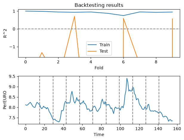

Five lags¶

OilExchange_train['PerEURO_lag2'] = OilExchange_train.PerEURO.shift(2).bfill()
OilExchange_train['PerEURO_lag3'] = OilExchange_train.PerEURO.shift(3).bfill()
OilExchange_train['PerEURO_lag4'] = OilExchange_train.PerEURO.shift(4).bfill()
OilExchange_train['PerEURO_lag5'] = OilExchange_train.PerEURO.shift(5).bfill()
OilExchange_train.head()

# Backtesting using sliding window with data
from sklearn.model_selection import cross_validate #       Negative indexing is scary!      -->
scores = cross_validate(pipe, pd.concat([OilExchange_train.loc[:, OilExchange_train.columns[3:-11]], 
                                         OilExchange_train[["PerEURO_lag1","PerEURO_lag2","PerEURO_lag3","PerEURO_lag4","PerEURO_lag5"]]], axis=1),
                                         OilExchange_train.loc[:, 'PerEURO'], cv=tscv_slide,
                                         scoring='r2', return_train_score=True)
scores

{'fit_time': array([0.00280404, 0.0025022 , 0.00299215, 0.0042491 , 0.00213289,
        0.00206828, 0.00184917, 0.00195408, 0.00385094, 0.00223804]),
 'score_time': array([0.00087714, 0.00094914, 0.00095701, 0.00236487, 0.00089097,
        0.00086474, 0.00082564, 0.00087094, 0.00119877, 0.00092983]),
 'test_score': array([-5.69820756e-01, -1.57221588e+00, -4.97861817e+00,  7.36545452e-02,
        -7.18201630e+00, -7.06614762e+02,  5.51939962e-01, -2.81878260e+00,
        -2.51922682e+00,  4.95828753e-01]),
 'train_score': array([1.        , 0.99248991, 0.96940659, 0.94583791, 0.95749656,
        0.91409406, 0.76327123, 0.97259431, 0.95439249, 0.96453061])}

# Plot the backtesting results for train and test data, and under it ad the original data (PerEURO) as a subplot
plt.subplot(2,1,1)
plt.plot(scores['train_score'], label='Train')
plt.plot(scores['test_score'], label='Test')
plt.xlabel('Fold')
plt.ylabel('R^2')
plt.title('Backtesting results')
plt.axhline(0, color='gray', linestyle='--')
plt.ylim(-1.6,1.1)
plt.legend()
plt.subplot(2,1,2)
plt.plot(OilExchange_train.loc[:, 'PerEURO'])
for i in range(10):
    plt.axvline(x=max_train[i], color='gray', linestyle='--')
plt.xlabel('Time')
plt.ylabel('PerEURO')
plt.show()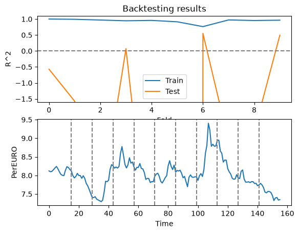

Correlation between time series¶

To get an impression of the connection between different variables, one can compute correlations, e.g., in the form of a correlation matrix.
If one expects one variable to affect another variable at a later time, correlation with a lag can be computed.
The degree of connection between two time series may also be dependent on time.
- A Sliding Window Correlation (SWC) shows local correlation in time windows.
- The window size (and possible lag) can be tuned for series of quick or slow changes.
Note: Correlation does not equal causation.
- There may not be a cause and effect, even though two phenomena show similar patterns. Beautifully illustrated by Tyler Vigen.
The concept of Autocorrelation will be covered later.

PerEURO_ExpNatGas_corr = np.corrcoef(OilExchange['PerEURO'], OilExchange['ExpNatGas'])
PerEURO_ExpNatGas_corr_lagged = np.corrcoef(OilExchange['PerEURO'][10:], OilExchange['ExpNatGas'][0:len(OilExchange['ExpNatGas'])-10])
print("Correlation between PerEURO and ExpNatGas: {:.3f}".format(PerEURO_ExpNatGas_corr[0,1]))
print("Correlation between PerEURO and ExpNatGas lagged 10 timepoints: {:.3f}".format(PerEURO_ExpNatGas_corr_lagged[0,1]))

Correlation between PerEURO and ExpNatGas: -0.000
Correlation between PerEURO and ExpNatGas lagged 10 timepoints: 0.093

# Use ipywidgets to create a slider for the lag
from ipywidgets import interact
def lagged_correlation(lag=0):
    x.index += lag
    corr = np.corrcoef(y[lag:], x[0:len(y)-lag])
    print("Correlation between {} and {} lagged {} timepoints: {:.3f}".format(x.name, y.name, lag, corr[0,1]))

x = OilExchange['ExpNatGas']
y = OilExchange['PerEURO']
interact(lagged_correlation, lag=(0,100,1)); # Semi-colon to suppress output

Correlation between ExpNatGas and PerEURO lagged 0 timepoints: -0.000

# Sliding window correlation with window size 45
PerEURO_ExpNatGas_SWC = OilExchange['PerEURO'].rolling(45, center=True).corr(OilExchange['ExpNatGas'])

# Plot PerEURO, ExpNatGas and PerEURO_ExpNatGas_SWC as subplots
def plot_SWC(center=22):
    plt.subplot(3,1,1)
    plt.plot(OilExchange['PerEURO'])
    plt.plot(range(center-22,center+22), OilExchange['PerEURO'][center-22:center+22], color="red")
    plt.ylabel('PerEURO')
    plt.xlim(0, len(OilExchange['PerEURO']))
    plt.subplot(3,1,2)
    plt.plot(OilExchange['ExpNatGas'])
    plt.plot(range(center-22,center+22), OilExchange['ExpNatGas'][center-22:center+22], color="red")
    plt.ylabel('ExpNatGas')
    plt.xlim(0, len(OilExchange['PerEURO']))
    plt.subplot(3,1,3)
    plt.plot(PerEURO_ExpNatGas_SWC)
    plt.plot(center, PerEURO_ExpNatGas_SWC[center], 'r.')
    plt.axhline(y=0, color='gray', linestyle=':')
    plt.ylim(-1,1)
    plt.xlim(0, len(OilExchange['PerEURO']))
    plt.xlabel('Time')
    plt.ylabel('SWC')
    plt.tight_layout()
    plt.show()

interact(plot_SWC, center=(22,len(OilExchange['PerEURO'])-23,1)) # Semi-colon to suppress output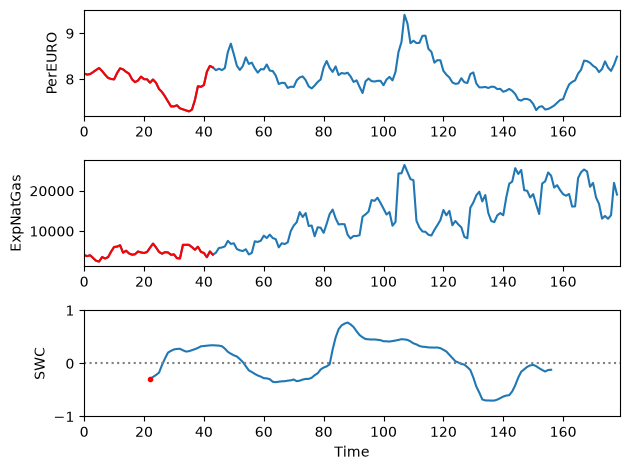

<function __main__.plot_SWC(center=22)>

Pandas’ rolling() and shifts¶

When applying Pandas’ rolling() function, the index is used for matching the data points.
Therefore, we need to shift the index of the ExpNatGas to achieve a lag.
Because of the sliding window, the two series do not need to match in length.

OE = OilExchange['ExpNatGas'].copy() # <- Remember to copy, to avoid changing the original data!
OE.index += 10
plt.plot(OilExchange['PerEURO'].rolling(45, center=True).corr(OE))
plt.xlim(0, len(OilExchange['PerEURO']))
plt.show()
OE.index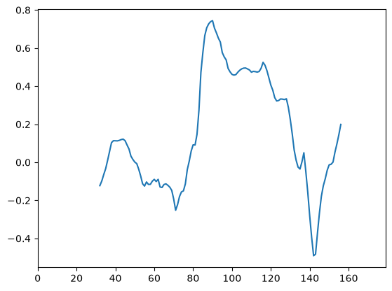

RangeIndex(start=10, stop=189, step=1)

Exercise¶

Combine lag and sliding window correlation.
Use ipywidgets to control:
- window width
- lag
- selected variable to compare to PerEURO
- bonus: visualize the sliding window like above