Pivot tables

# Read SalesData.xlsx
import pandas as pd
df = pd.read_excel('../../data/SalesData.xlsx', skiprows=4, header=0)
print(df.shape)
df.head()

# Add a column giving the total price
df['TotalPrice'] = df['Quantity'] * df['UnitPrice']
df.head()

# Use Pandas groupby() to group by Channel and sum the TotalPrice
df1 = df.groupby('Channel')['TotalPrice'].sum()
df1

# Use Pandas pivot_table() to group by Channel and Manager and sum the TotalPrice
df2 = df.pivot_table(index='Channel', columns='Manager', values='TotalPrice', aggfunc='sum')
df2

# Exchange aggfunc='sum' for aggfunc='count' to confirm that the dataset is not very suitable for this type of analysis
df2 = df.pivot_table(index='Channel', columns='Manager', values='TotalPrice', aggfunc='count')
df2

# Read the athlete_events.csv file
import pandas as pd
athletes = pd.read_csv('../../data/athlete_events.csv')
print(athletes.shape)
athletes.head()

# Check average weight of athletes
athlete_weight = athletes['Weight'].mean()

# Print athlete_weight with 2 decimal places and kg suffix
print('Average weight of athletes: {:.2f} kg'.format(athlete_weight))

# Check average weight of athletes for each year
athlete_weight_by_year = athletes.groupby('Year')['Weight'].mean()

# Plot athlete_weight_by_year using kind='bar'
import matplotlib.pyplot as plt
athlete_weight_by_year.plot(kind='bar', figsize=(12, 4))
# Add horizontal grid lines to the plot
plt.grid(axis='y') 
plt.show()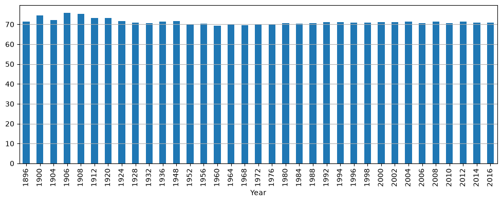

# Check average weight of athletes for each sport and drop NA values
athlete_weight_by_sport = athletes.groupby('Sport')['Weight'].mean().dropna()
athlete_weight_by_sport

# Make a pivot table of athlete weights by sport and year
athlete_weight_sport_year = athletes.pivot_table(index='Sport', columns='Year', values='Weight', aggfunc='mean')
athlete_weight_sport_year

# Extract the rows for Season == Summer and Year >= 2000
summer = athletes.loc[athletes['Season'] == 'Summer',:]
summer2000 = summer.loc[summer['Year'] >= 2000,:]
summer2000.head()

# Repeat the pivoting step on the summer2000 data
awsy = summer2000.pivot_table(index='Sport', columns='Year', values='Weight', aggfunc='mean')

# Remove rows that only contain NaN values
awsy = awsy.dropna(how='all')
awsy.round(1)

# Repeat, but limit to summers of 2000-2016
awsy = summer2000.pivot_table(index='Sport', columns='Year', values=['Weight','Height'], aggfunc=['mean','max'])

# Remove rows that only contain NaN values
awsy = awsy.dropna(how='all')
awsy.round(1).head()

# Repeat, but add margins
awsy = summer2000.pivot_table(index='Sport', columns='Year', values=['Weight','Height'], aggfunc='max', margins=True)

# Remove rows that only contain NaN values
awsy = awsy.dropna(how='all')
awsy.round(1).head()

# Groupby with two columns
athlete_weight_by_sport_groupby = athletes.groupby('Sport')[['Weight','Height']].mean()
athlete_weight_by_sport_groupby

# Unstack the result
athlete_weight_by_sport_groupby.unstack()