Outlier statistics - Data to Decision

Determining if a sample or timepoint is a statistical outlier is often a two-step process:
1. Estimate a distribution assumed to be normal operating conditions.
2. Check if new samples are significant outliers from this distribution.
(Multivariate) Statistical Process Control, part of $6\sigma$ process improvement, has a wide range of methods for this.

Statistical Process Control - SPC¶

The simplest form handles a single variable.
A normal distribution is assumed, but some deviation is tolerated.
It also assumes a constant/stationary process and no shifts/trends in distributions.
Any value outside +/- 3 standard deviations (SD) of the mean is assumed to be an outlier.

# Plot the normal probability curve from -4 to 4 with mean 0 and standard deviation 1
import numpy as np
import scipy.stats as stats
import matplotlib.pyplot as plt
plt.figure(figsize=(5,3))
x = np.linspace(-4, 4, 100)
y = stats.norm.pdf(x, 0, 1)
plt.plot(x, y, color='black')
plt.xlabel('Standard deviations')
plt.ylabel('Probability density')
plt.title('Standard normal probability curve')
# Shade the area under the curve to the left of -3 and right of 3
px = np.linspace(-4, -3, 100)
py = stats.norm.pdf(px, 0, 1)
plt.fill_between(px, py, color='red')
px = np.linspace(3, 4, 100)
py = stats.norm.pdf(px, 0, 1)
plt.fill_between(px, py, color='red')
plt.show()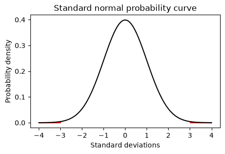

# Calculate the probability of being outside +/- 3 SD in a normal distribution, i.e. P(|X| > 3).
# Format the result as a percentage rounded to two decimal places.
import scipy.stats as stats
prob = stats.norm.cdf(-3)*2
print('Probability of being outside +/- 3 SD in a normal distribution: {:.2%}'.format(prob))
# Rewrite this as the proportion of values, i.e., 1 in n, that are outside +/- 3 SD in a normal distribution.
print('Proportion of values that are outside +/- 3 SD in a normal distribution: 1 in {:.0f}'.format(1/prob))

Probability of being outside +/- 3 SD in a normal distribution: 0.27%
Proportion of values that are outside +/- 3 SD in a normal distribution: 1 in 370

Control charts¶

A common way of assessing outliers is to plot the series together with lower and upper boundaries.

# Plot random normal data with 1000 values with a seed of 1
import numpy as np
np.random.seed(1)
data = np.random.normal(0, 1, 1000)
plt.figure(figsize=(10,3))
plt.plot(data, 'o')
plt.ylim(-4.5, 4.5)
plt.xlim(0, 1000)
plt.axhline(0, color='black', linestyle='--')
plt.axhline(3, color='red')
plt.axhline(-3, color='red')
plt.ylabel('Standard deviations')
plt.xlabel('Observations')
# Plot all samples that are outside +/- 3 SD in a normal distribution in red
outliers = data[np.abs(data) > 3]
plt.plot(np.where(np.abs(data) > 3)[0], outliers, 'o', color='red')
plt.show()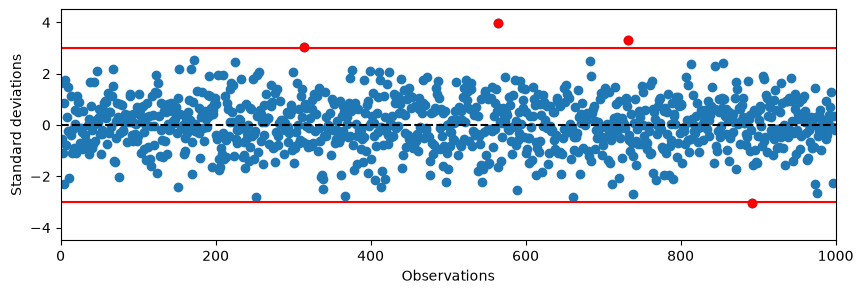

Histograms¶

Histograms show you a cummulative view over a set of observations.
If the observed distribution is very different from a bell curve (normal distribution), the +/-3 SD will not have the expected coverage.
- Associated P-values will be wrong.

# Plot the same data as a histogram
plt.figure(figsize=(5,3))
plt.hist(data, bins=50)
plt.ylabel('Frequency')
plt.xlabel('Standard deviations')
plt.title('Histogram of random normal data')
plt.axvline(3, color='red')
plt.axvline(-3, color='red')
plt.show()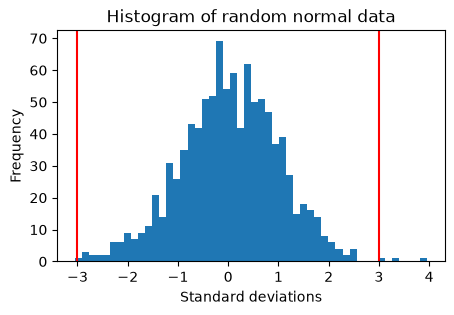

# Calculate the probability of observing a value more extreme 
# than the maximum absolute value in the data set at random
stats.norm.sf(np.max(np.abs(data)))*2

np.float64(7.538952188296564e-05)

Quantile plots¶

A quantile plot plots expected quantiles of a distributon against observed quantiles from data.
The basic distribution is the normal probability distribution.

# A quantile plot can also help to identify outliers and deviations from normality
plt.figure(figsize=(4,3))
stats.probplot(data, dist='norm', plot=plt)
plt.show()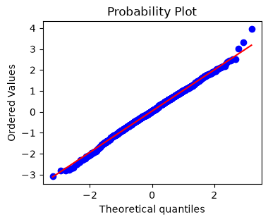

Robust statistics¶

Instead of mean and standard deviation, one can use more robust calculations.
Trimmed mean means first removing a proportion, e.g., 5% of the most extreme observations before calculating the mean.
- Robust against outliers.
Median absolute deviation is the median of the absolute deviations from the median value.
- Robust against non-normality.

MAD = median(|X_i - \tilde{X}|), ~~~ \tilde{X} = median(X)

(1)

Relation to standard deviation: $\hat{\sigma} = k \cdot MAD$ .
For normal data $k \approx 1.4826$ , see Wikipedia.

# Trimmed mean
m1 = np.mean(data)
m2 = stats.trim_mean(data, 0.05)
print('Mean: {:.3f}'.format(m1))
print('Trimmed mean: {:.3f}'.format(m2))

Mean: 0.039
Trimmed mean: 0.046

# Median absolute deviation
s1 = np.std(data)
s2 = stats.median_abs_deviation(data)
print('Standard deviation: {:.3f}'.format(s1))
print('Median absolute deviation: {:.3f}'.format(s2))

Standard deviation: 0.981
Median absolute deviation: 0.647

# SD vs MAD
print('Adjusted MAD: {:.3f}'.format(s2 * 1.4826))

Adjusted MAD: 0.959

Heuristics¶

As seen above, to be flagged in the base case will happen by accident 1 in 370 cases.
The probability quickly shrinks if additional requirements are added, e.g., 3 cases in a row outside +/- 3 std.
- With multiple consecutive outliers, one can also use fewer standard deviations.
If data are assumed to be iid (independent and identically distributed), another heuristic can be to check if concecutive samples are too similar (and possibly non-centred).
- This can indicate a bias in the series, e.g., caused by a manufacturing step caught in an error condition.
A shift in mean value can also be indicative of errors or unwanted changes; checkable using rolling means or similar with an appropriate window size.
- A whole field of SPC uses Exponentially Weighted Moving Averages to detect outliers and shifts in distributions.

# Assuming independent samples, calculate the probability of observing
# three values in a row above 2 SD in a normal distribution.
prob3 = (1-stats.norm.cdf(2))**3
print('Probability: {:.4%}'.format(prob3))
print('Proportion: 1 in {:.0f}'.format(1/prob3))

Probability: 0.0012%
Proportion: 1 in 84927

# Create a function that checks if n consecutive samples are above k SD or below -k SD
def check_consecutive(data, k, n, mu, SD):
    index = []
    dataUp = (data-mu) > k*SD
    dataDown = (data-mu) < -k*SD
    for i in range(len(data)-n+1):
        if np.all(dataUp[i:i+n]) or np.all(dataDown[i:i+n]):
            index.append(i)
    return index

# Apply hueristic function and plot
k = 2
n = 2
mu = 0
SD = 1
index = check_consecutive(data, k, n, mu, SD)

plt.figure(figsize=(10,3))
plt.plot(data, 'o')
plt.ylim(-4.5, 4.5)
plt.xlim(0, 1000)
plt.axhline(0, color='black', linestyle='--')
plt.axhline(k*SD, color='red')
plt.axhline(-k*SD, color='red')
plt.ylabel('Standard deviations')
plt.xlabel('Observations')
# Plot all samples that are caught by the heuristic function
for i in index:
    plt.plot(range(i,i+n), data[range(i,i+n)], 'o', color='yellow')
plt.show()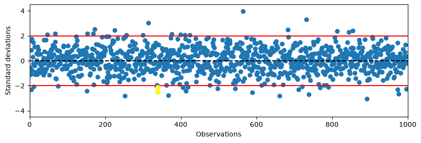

Exercise¶

Import the data called bananas.csv.
Assume the first 500 samples are “in control” and calculate their mean and standard deviation.
Plot the whole series and indicate outliers using SPC and heuristics.

Multivariate series¶

Though each variable can be handled separately with SPC, it is often more interesting to assess the combined effect.
Smaller deviations in single variables may be detected if these occur in relation to other variables and their variation.
Instead of the normal distribution, we use Mahalanobis distance and the associated Hotelling’s $T^2$ , a multivariate generalisation of the student t-distribution. $t^2$ is defined as:

t^2 = (\bar{x}-\mu) \hat{\Sigma}_{\bar{x}}^{-1} (\bar{x}-\mu)^T

(2)

In practice we estimate $\mu$ and $\hat{\Sigma}_{\bar{x}}$ from “in control” data and look at single observations for $\bar{x}$ , i.e., $x$ .

\frac{n-p}{p(n-1)}t^2 \sim F_{p,n-p}

(3)

where $n$ is the number of samples in the training data and $p$ is the number of variables.

# Read the Beijing pollution data
import pandas as pd
pollution = pd.read_csv("../../data/pollution.csv", header=0, index_col=0)
# Extract the first 2000 samples of DEWP, TEMP and PRES
pdata = pollution[['DEWP', 'TEMP', 'PRES']].iloc[:2000]

# Plot the three variables as separate subplots above each other
plt.figure(figsize=(10,6))
plt.subplot(311)
plt.plot(pdata['DEWP'], '-')
plt.ylabel('DEWP')
plt.subplot(312)
plt.plot(pdata['TEMP'], '-')
plt.ylabel('TEMP')
plt.subplot(313)
plt.plot(pdata['PRES'], '-')
plt.ylabel('PRES')
plt.xlabel('Observation')
plt.show()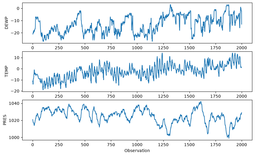

We use the first three years as the “in control” region and estimate mean and covariance from it.

# Calculate the mean vector and covariance matrix of the three variables for the first 3 years
import numpy as np
mean = np.mean(pdata.values[:365*3,:], axis=0)
cov = np.cov(pdata.values[:365*3,:], rowvar=False)
print(mean)
print(cov)

[ -16.62009132   -5.42648402 1028.2803653 ]
[[ 33.50636014   8.27369045 -16.68247894]
 [  8.27369045  27.0510347  -12.9269373 ]
 [-16.68247894 -12.9269373   32.5255282 ]]

# Calculate the Hotelling's T^2 statistic for each observation given mu and cov
def Hotellings_T2(X, mean, cov, n, alpha = 0.01):
    T2 = np.sum(((X-mean) @ np.linalg.inv(cov)) * (X-mean), axis=-1)
    p = len(mean)
    F = (n-p)/(p*(n-1))*T2
    P = stats.f.sf(F, p, n-p)
    # Critical value
    c = stats.f.isf(alpha, p, n-p)*p*(n-1)/(n-p)
    return (T2, F, P, c)

# Apply Hotellings_T2 and plot
alpha = 0.0027
T2, F, P, c = Hotellings_T2(pdata.values, mean, cov, 365*3, alpha)
plt.figure(figsize=(10,6))
plt.subplot(211)
plt.plot(T2)
plt.grid()
plt.axhline(c, color="red")
plt.axvline(365*3, color="orange")
plt.ylabel("T2")
plt.subplot(212)
# Plot P on a logarithmic scale
plt.plot(P)
plt.yscale("log")
plt.grid()
plt.axhline(alpha, color="red")
plt.axvline(365*3, color="orange")
plt.ylabel("P-value")
plt.xlabel("Observation")
plt.show()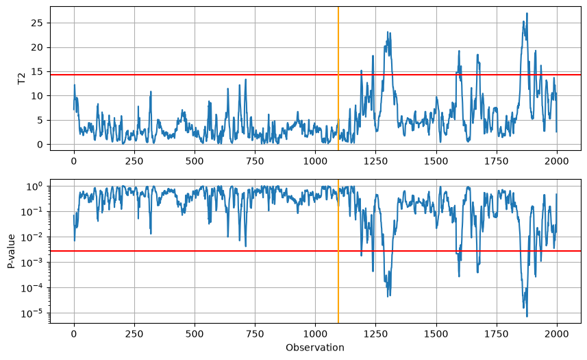

Finally, we observe which observations are marked as outlying in the original series.

# Plot the three variables as separate subplots above each other, marking the outlying regions in red
x = np.arange(2000)+0.0
x[P>alpha] = np.nan

plt.figure(figsize=(10,6))
plt.subplot(311)
plt.plot(pdata['DEWP'], '-')
plt.plot(x, pdata['DEWP'], '-', color='red')
plt.ylabel('DEWP')
plt.subplot(312)
plt.plot(pdata['TEMP'], '-')
plt.plot(x, pdata['TEMP'], '-', color='red')
plt.ylabel('TEMP')
plt.subplot(313)
plt.plot(pdata['PRES'], '-')
plt.plot(x, pdata['PRES'], '-', color='red')
plt.ylabel('PRES')
plt.xlabel('Observation')
plt.show()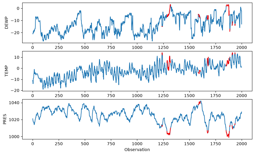

Robust multivariate statistics¶

Also multivariate data can need robust statistics because of non-normality or outliers.
One method for robust estimation of mean and standard deviation is called Minimum Covariance Determinant (MCD).
MCD uses a subset of samples that minimises the determinant of the covariance matrix.
An iterative method that searches for the MCD is implemented in scikit-learn’s MinCovDet.

# Import Minimum Covariance Determinant estimator from scikit-learn
from sklearn.covariance import MinCovDet
# Apply the Minimum Covariance Determinant estimator to data.values[:365*3,:] and plot
some_data = np.random.multivariate_normal(mean, cov, 10)
mcd = MinCovDet(random_state=1).fit(some_data)
mcd_mean = mcd.location_
mcd_cov = mcd.covariance_
mcd2 = MinCovDet(random_state=3).fit(pdata.values)
mcd2_mean = mcd2.location_
mcd2_cov = mcd2.covariance_

print(mcd_mean)
print(mcd_cov)
print(mcd2_mean)
print(mcd2_cov)
print(mean)
print(cov)

[ -14.55375772   -4.724472   1025.94736149]
[[ 42.75733002  21.71212165 -10.4415423 ]
 [ 21.71212165  44.64007986 -32.03879093]
 [-10.4415423  -32.03879093  25.19171101]]
[ -13.52995928   -2.41361257 1026.06748109]
[[ 50.39563984  16.364267   -33.07242179]
 [ 16.364267    31.89569218 -24.36020609]
 [-33.07242179 -24.36020609  48.7317869 ]]
[ -16.62009132   -5.42648402 1028.2803653 ]
[[ 33.50636014   8.27369045 -16.68247894]
 [  8.27369045  27.0510347  -12.9269373 ]
 [-16.68247894 -12.9269373   32.5255282 ]]

Exercise¶

Repeat the calculations of mean, covariance, Hotelling’s $T^2$ , etc. for the Beijing pollution data.
Exchange ordinary statistics with the MCD alternative.

Time resolution¶

The (M)SPC examples have assumed a constant mean and standard deviation.
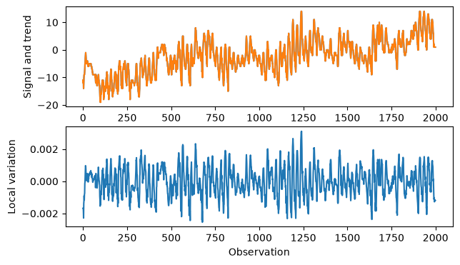
It may also be interesting to look at det deviation from smoothed data to look for local outliers.
- This corresponds to a high-pass filter for FFT.
In the rich field of (M)SPC there are also other methods tailored for finding shifts in trends.

from scipy.fft import dct, idct
fourier_signal = dct(pdata["TEMP"].values, type=1, norm="forward")

# Plot the Fourier transform
plt.figure(figsize=(7,2))
plt.plot(np.abs(fourier_signal))
plt.xlabel('Frequency')
plt.ylabel('Fourier Transform')
plt.show()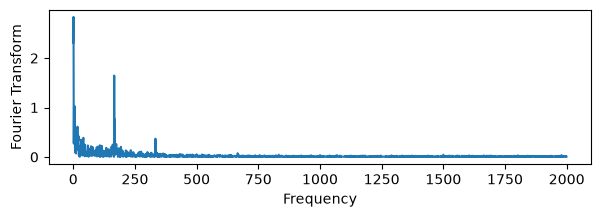

# Filter the Fourier transform by setting all frequencies below a threshold to zero
W = np.arange(0, 2000) # Frequency axis
filtered_fourier_signal = fourier_signal.copy()
filtered_fourier_signal[(W<30)] = 0
cut_signal = idct(filtered_fourier_signal)

# Plot the filtered signal
plt.figure(figsize=(7,4))
plt.subplot(211)
plt.plot(pdata["TEMP"].values)
plt.plot(pdata["TEMP"].values - cut_signal)
plt.ylabel('Signal and trend')
plt.subplot(212)
plt.plot(cut_signal)
plt.ylabel('Local variation')
plt.xlabel('Observation')
plt.show()