Decomposition - Data to Decision

There are various regimes for signal decomposition.
Examples:
- Fast Fourier Transform (FFT)
- Wavelets
- Linear components
Motviation:
- Trend discovery
- Low-pass/high-pass filter
- Exploratory data analysis

Fast Fourier Transform¶

FFT history and application¶

An important workhorse in signal processing.
Can be traced back to Carl Friedrich Gauss on Discrete Fourier Transforms from 1805.
Major milestone in 1965 by James Cooley and John Tukey regarding speed of computations and applications in detecting Soviet nuclear bomb tests.
Used in anything from mathematical speed-ups, via video and music compression, modern signal processing in Wi-Fi, 5G, etc. to finance.

FFT function¶

Wikipedia: A Fourier Transform is a transform that converts a function into a form that describes the frequencies present in the original function.
scipy.fft: Fourier analysis is a method for expressing a function as a sum of periodic components, and for recovering the signal from those components.

X_k = \sum_{n=0}^{N-1} x_n e^{i2 \pi kn/N} ~~~~ k = 0, ..., N-1

(1)

Here, k is the index of a signal, X, and N is its length. $x_n$ is a coefficient to be fitted.

import numpy as np
import matplotlib.pyplot as plt
N = 100
n = 1
x = [np.exp(1j * 2 * np.pi * k * n / N) for k in range(N)]
plt.plot(range(N), np.real(x), '.')
plt.ylabel('Real part')
plt.show()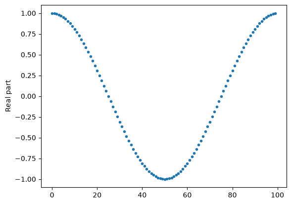

# The full complex exponential basis
plt.plot(np.real(x), np.imag(x), '.')
plt.axis('square')
plt.grid()
plt.xlabel('Real')
plt.ylabel('Imaginary')
plt.title('DFT Basis')
plt.show()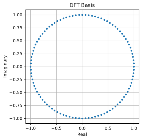

Direct Cosine Transform (DCT)¶

FFT with real valued data.
For real numbered signals, the definition above can be exchanged with a version based on the cosine or sine functions.
There are theoretically 8+8 “types”, 4+4 of which are implemented in SciPy, and various choices for normalisation.
Type I DCT (Direct Cosine Transform) as implemented in SciPy:

y_k = x_0 + (-1)^k x_{N-1} + 2 \sum_{n=1}^{N-2} x_n cos (\frac{\pi k n}{N-1}))

(2)

$y_k$ is the $k$ -th part of the signal, $N$ is the length, $x_n$ is the $n$ -th coefficient.
Coefficient signs indicate flip of the base cosines, magnitudes indicate scaling.
n indicates the number of half cosine cycles, i.e., even n means full cycles (see plot below), maximum frequency of n/2.
Quicker than FFT and guarantees real valued frequency domain.

N = 100
n = 3
for k in range(0,n+1):
    plt.plot(np.cos(np.pi*k*np.arange(N)/(N-1)), label='n='+str(k))
plt.title('DCT Basis')
plt.xlabel('k')
plt.legend()
plt.show()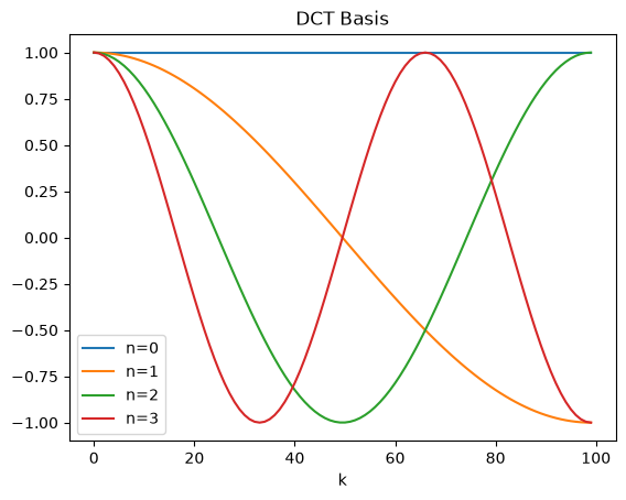

# Sum of two cosines with different frequencies.
import numpy as np
from scipy.fft import dct, idct

N = 601
s = 3
time = np.linspace(0,s,N)
s3 = np.cos(3 * 2*np.pi * time)
s5 = np.cos(5 * 2*np.pi * time)
signal = s3 + s5

# Make three suplots above each other with s3, s5 and signal
fig, axs = plt.subplots(3, 1, figsize=(7, 5))
axs[0].plot(time, s3)
axs[0].set_title('s3')
axs[1].plot(time, s5)
axs[1].set_title('s5')
axs[2].plot(time, signal)
axs[2].set_title('signal')
for ax in axs.flat:
    ax.set(xlabel='Time (s)', ylabel='Signal')
plt.tight_layout()
plt.show()

# Print the resolution of the time axis in Hz
dt = time[1] - time[0]
print('Sampling of the time axis:', 1/dt, 'Hz')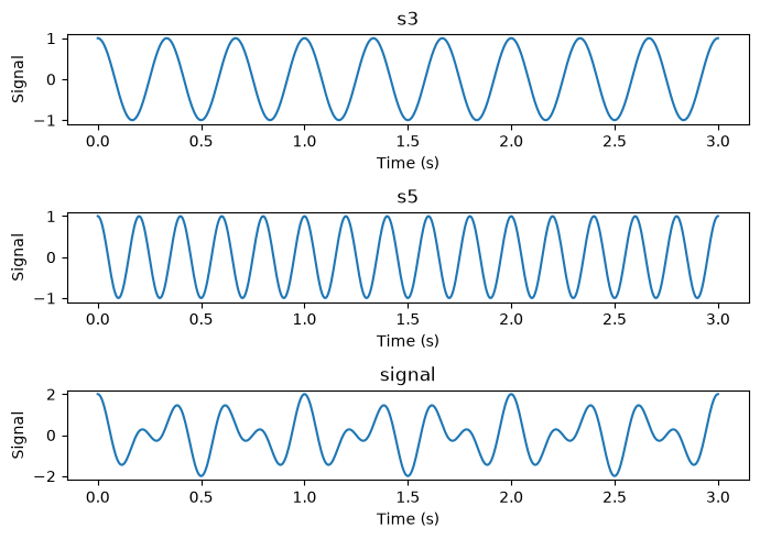

Sampling of the time axis: 200.0 Hz

# Discrete Cosine transform
shift = 0 # Shift the signal to the right by this amount, e.g., 100
fourier_signal = dct(np.concatenate([np.zeros(shift),signal]), type=1, norm="forward") # Pad with zeros to shift signal
dt = time[1] - time[0]
W = np.linspace(0, 1/(2*dt), N+shift)
#                    ^-- Frequency axis in Hz (2* because of of definitions of DCT with half integers)

# Plot the Fourier transform
fig, axs = plt.subplots(2, 1, figsize=(7, 4))
axs[0].plot(range(N+shift), fourier_signal)
axs[0].set_xlabel('Coefficient')
axs[0].set_ylabel('Fourier Transform')
axs[0].set_xlim(0, N+shift)
axs[1].plot(W, fourier_signal)
axs[1].set_xlabel('Frequency (Hz)')
axs[1].set_ylabel('Fourier Transform')
axs[1].set_xlim(0, np.max(W))
plt.tight_layout()
plt.show()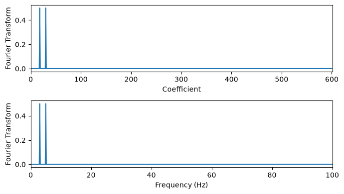

FFT filtering¶

We can apply the FFT to analyse the frequencies present or to filter the signal.
- Filtering here means that some frequencies are removed from the signal.
Typical filters are:
- Low-pass filter: Remove high frequencies, e.g., noise or short-term changes, focusing on trends or slowly changing signals.
- High-pass filter: Remove low frequencies, e.g., trends or baselines, focusing on rapid changes or anomalies.

plt.plot(W)
plt.show()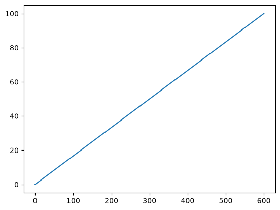

# Remove frequencies below 4, i.e., a high-pass filter
filtered_fourier_signal = fourier_signal.copy()
filtered_fourier_signal[(W<4)] = 0 # <- Come play with me!
cut_signal = idct(filtered_fourier_signal, type=1, norm="forward")

# Plot the filtered signal
plt.figure(figsize=(7,2))
plt.plot(time, cut_signal)
plt.xlabel('Time')
plt.ylabel('Filtered Signal')
plt.xlim(0,s)
plt.axhline(-1, color='k', alpha=0.5, linewidth=0.5) # Shows the inexactness of the reconstruction
plt.axhline(1, color='k', alpha=0.5, linewidth=0.5)
plt.show()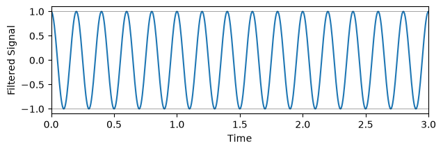

# A curve we have seen before
N = 301
rng = np.random.default_rng(0)
y = rng.standard_normal(N).cumsum()

# Plot the curve
plt.figure(figsize=(7,3))
plt.plot(y)
plt.xlabel('arbitrary units')
plt.ylabel('amplitude')
plt.show()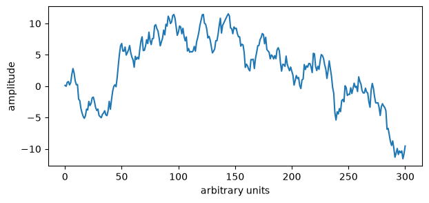

# Plot the Fourier transform
plt.figure(figsize=(7,3))
plt.plot(np.abs(dct(y, type=1, norm="forward"))) # Not caring about the signs
#plt.plot(dct(y, type=1)) # Caring about the signs
plt.xlabel('coefficient')  # Think 1/width of time series
plt.ylabel('amplitude')
plt.xlim(0,N)
plt.show()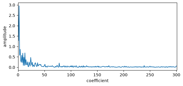

Overlay cosines on signal¶

# Remove frequencies above 50, i.e., a low-pass filter.
W = np.arange(0, N) # Frequency axis
filtered_fourier_signal = dct(y, type=1, norm="forward")
x = filtered_fourier_signal.copy()
filtered_fourier_signal[(W > 10)] = 0
cut_signal = idct(filtered_fourier_signal, type=1, norm="forward")
add_cosines = 3 # <- Change me! Non-negative number adds cosines to the filtered signal

# Plot the filtered signal
plt.figure(figsize=(7,3))
plt.plot(y)
plt.plot(cut_signal)
plt.xlabel('arbitrary units')
plt.ylabel('amplitude')
plt.xlim(0,N)
if add_cosines > -1:
    for k in range(0,add_cosines+1):
        plt.plot(2 * x[k] * np.cos(np.pi*k*np.arange(N)/(N-1)) * 2) # Scaled up by 2 to fit in plot
plt.show()
#print('Sum of original signal: {:.2f}'.format(np.sum(y)))
#print('0th DCT coefficient / 2: {:.2f}'.format(filtered_fourier_signal[0]/2)) # Only holds for type 2 DCT with norm="backward"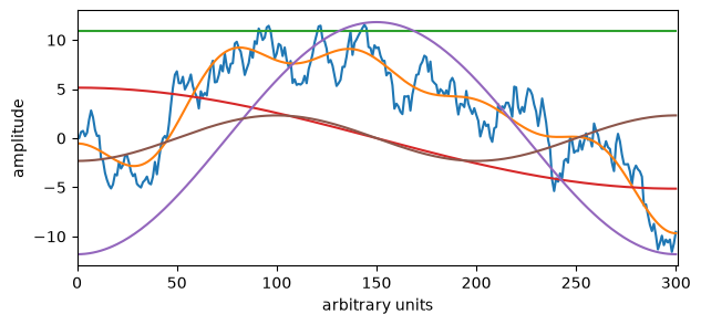

y_k = x_0 + (-1)^k x_{N-1} + 2 \sum_{n=1}^{N-2} x_n cos (\frac{\pi k n}{N-1}))

(3)

Linear decomposition¶

Various forms of linear models can be used for decomposition, each having different focus or optimality criteria, e.g.:
- Seasonal-Trend decomposition using LOESS in the statmodels package
- Multivariate explorative data analysis with Principal Component Analysis.

Seasonal-Trend decomposition using LOESS (STL)¶

STL takes a (time) series as input together with an estimate of period length.
Output are:
- A trend along the series (T).
- A seasonal signal which may evolve along the series (S).
- A residual (R).
- Additive: X = T + S + R
- (Multiplicative: X = T * S * R)
Additional parameters:
- Length of smoothers for trend and season (high number = less change).
- Use weighting of samples for robustness (allow more individual deviation from trend/season).

Fitting:

Simplified, one can think of STL is being fitted one component at a time.
- Smooth the series to estimate the trend,
  $T = f_{smooth,T}(X)$ .
- Subtract the trend from the series,
  $X_{S+R} = X - T$ .
- Average across seasons with sliding window (LOESS) to estimate the season,
  $S = f_{smooth,S}(X_{S+R})$ .
- Subtract the trend and season from the signal to estimate the residual,
  $R = X - T - S$
In practice, this happens within a loop where observations are given weights which are updated iteratively based on previous fits.

# Monthly sunspots from https://github.com/jbrownlee/Datasets

# Load the data
import pandas as pd
sunspots = pd.read_csv("../../data/monthly-sunspots.csv", header=0)
print(sunspots.shape)
sunspots.head()

(2820, 2)

# Plot the data
sunspots.plot.line(x='Month', y='Sunspots', figsize=(7,2))
plt.xlabel('Month')
plt.ylabel('Number of sunspots')
plt.show()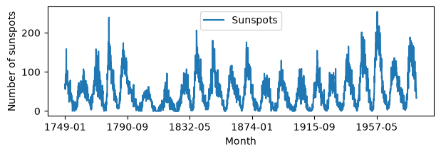

# Approximate periodicity: Lenght of series divided by number of periods.
# For sunspots we know that there is a periodicity of approximately 11 years.
np.round(2820/21)

np.float64(134.0)

from statsmodels.tsa.seasonal import STL
stl = STL(sunspots["Sunspots"], period=134)#, robust=True, seasonal=141, trend=141)
res = stl.fit() # Contains the components and a plot function
fig = res.plot()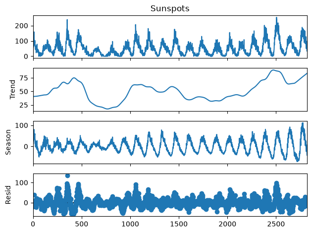

# Daily Female Births in California from https://github.com/jbrownlee/Datasets

# Load the data
births = pd.read_csv("../../data/daily-total-female-births.csv", header=0)
births.head()

stl = STL(births["Births"], period=30)
res = stl.fit()
fig = res.plot()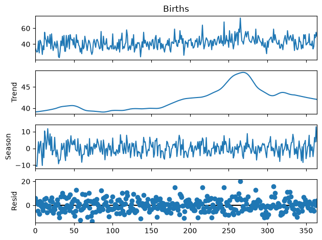

Excercise¶

Force the period to change less.
Extract the trend and plot it as a function of time.
Indicate the date of maximum number of conceptions (~9 months before birth), assuming the year is cyclic.

Multiple seasonalities¶

If a there is more than one phenomenon with a cyclic behaviour, multiple seasonalities can be found through Multiple Seasonal-Trend decomposition using LOESS (MSTL).
The more complex model one applies, the higher the chances of overfitting!
Example at statsmodels.org

Principal Component Analysis (PCA)¶

For (time) series with multiple variables, PCA can give a first indication of structure and connection between variables.
Scores show paths of time points, loadings show how variables relate.
One PCA formulation for input data $\mathbf{X}$ with series as columns:

\mathbf{U} \mathbf{S} \mathbf{V}' = svd(\mathbf{X}-\bar{\mathbf{X}})

(4)

\mathbf{T} = \mathbf{U} \mathbf{S} \text{ - scores}

(5)

\mathbf{P} = \mathbf{V}' \text{ - loadings}

(6)

Beijing pollution data¶

This dataset is originally from UCI Machine Learning Repository and shows hourly measurements of weather at the US embassy in Bejing. Its columns are:

No: row number
year: year of data in this row
month: month of data in this row
day: day of data in this row
hour: hour of data in this row
pm2.5: PM2.5 concentration ( $\mu g/m^3$ )
DEWP: Dew Point ( $^{\circ}F$ )
TEMP: Temperature ( $^{\circ}F$ )
PRES: Pressure (hPa)
cbwd: Combined wind direction
Iws: Cumulated wind speed
Is: Cumulated hours of snow
Ir: Cumulated hours of rain

# Beijing pollution data from https://github.com/jbrownlee/Datasets

# Load the data
pollution = pd.read_csv("../../data/pollution.csv", header=0, index_col=0)
print(pollution.shape)
pollution.head()

(43824, 12)

# Recode the cbwd column using one-hot encoding and add to the data frame
pollution = pd.concat([pollution, pd.get_dummies(pollution["cbwd"], dtype=float)], axis=1)
pollution = pollution.drop(columns=["cbwd"])
pollution.head()

# Replace NaN with 0 in the pm2.5 column
pollution["pm2.5"] = pollution["pm2.5"].fillna(0)
pollution.head()

# PCA of pollution data
from hoggorm.pca import nipalsPCA as PCA
pca = PCA(pollution.iloc[:,4:].values, numComp=4, Xstand=True)

# Make a 2D histogram of the X_scores (too many points for a scatter plot)
plt.figure(figsize=(4,4))
plt.hist2d(pca.X_scores()[:,0], pca.X_scores()[:,1], bins=200)
plt.xlabel("PC 1")
plt.ylabel("PC 2")
plt.show()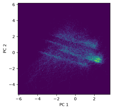

# Loading plot
from hoggormplot import loadings
loadings(pca, comp=[1,2], XvarNames=pollution.columns[4:].tolist())
plt.show()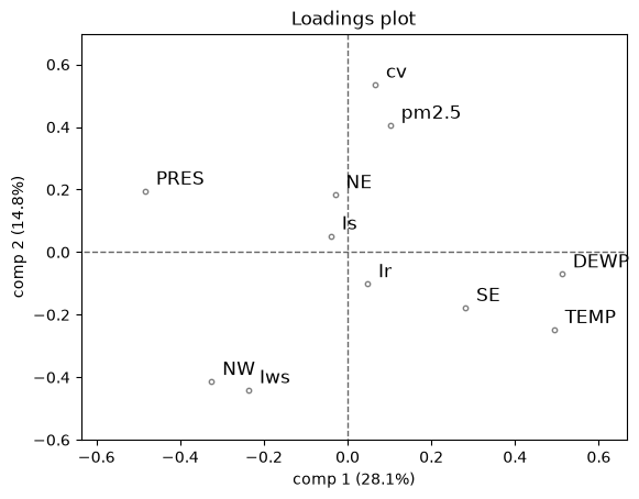

# Make a 2D histogram of the X_scores (too many points for a scatter plot)
plt.figure(figsize=(4,4))
plt.hist2d(pca.X_scores()[:,0], pca.X_scores()[:,1], bins=200)
plt.xlabel("PC 1")
plt.ylabel("PC 2")
labs = pollution.columns[4:].tolist()
# Add an axis cross in gray using axhline and axvline
plt.axhline(0, color="gray")
plt.axvline(0, color="gray")
# Add the loadings as text (labs) in white on top of the histogram, scale to the same range as the histogram
for i in range(len(labs)):
    plt.text(pca.X_loadings()[i,0]*4, pca.X_loadings()[i,1]*4, labs[i], color="white")
plt.show()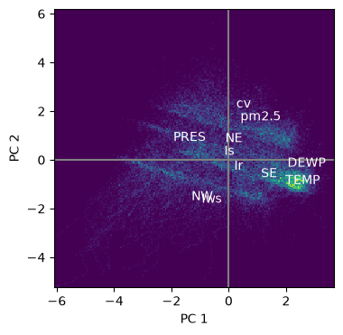

# Plot the 3rd and 4th components
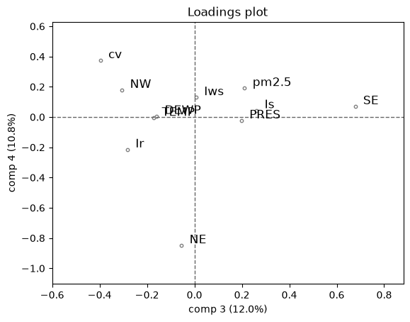
loadings(pca, comp=[3,4], XvarNames=pollution.columns[4:].tolist())
plt.show()