Plots of Scores, Loadings and Correlation Loadings

Functions to make scatter plots of scores or correlation loadings, and scatter or line plots of loadings.

Usage

scoreplot(object, ...)

# Default S3 method
scoreplot(
  object,
  comps = 1:2,
  labels,
  identify = FALSE,
  type = "p",
  xlab,
  ylab,
  estimate,
  newdata,
  ...
)

# S3 method for class 'scores'
plot(x, ...)

loadingplot(object, ...)

# Default S3 method
loadingplot(
  object,
  comps = 1:2,
  scatter = FALSE,
  labels,
  identify = FALSE,
  type,
  lty,
  lwd = NULL,
  pch,
  cex = NULL,
  col,
  legendpos,
  xlab,
  ylab,
  pretty.xlabels = TRUE,
  xlim,
  ...
)

# S3 method for class 'loadings'
plot(x, ...)

corrplot(
  object,
  comps = 1:2,
  labels,
  plotx = TRUE,
  ploty = FALSE,
  radii = c(sqrt(1/2), 1),
  identify = FALSE,
  type = "p",
  xlab,
  ylab,
  col,
  ...
)

Arguments

object: an object. The fitted model.
...: further arguments sent to the underlying plot function(s).
comps: integer vector. The components to plot.
labels: optional. Alternative plot labels or \(x\) axis labels. See Details.
identify: logical. Whether to use identify to interactively identify points. See below.
type: character. What type of plot to make. Defaults to "p" (points) for scatter plots and "l" (lines) for line plots. See plot for a complete list of types (not all types are possible/meaningful for all plots).
xlab, ylab: titles for \(x\) and \(y\) axes. Typically character strings, but can be expressions or lists. See title for details.
estimate: optional character vector passed to scores() so scoreplot() can request the training, CV or test estimate when plotting.
newdata: optional data frame supplied to scores() when estimate = "test".
x: a scores or loadings object. The scores or loadings to plot.
scatter: logical. Whether the loadings should be plotted as a scatter instead of as lines.
lty: vector of line types (recycled as neccessary). Line types can be specified as integers or character strings (see par for the details).
lwd: vector of positive numbers (recycled as neccessary), giving the width of the lines.
pch: plot character. A character string or a vector of single characters or integers (recycled as neccessary). See points for all alternatives.
cex: numeric vector of character expansion sizes (recycled as neccessary) for the plotted symbols.
col: character or integer vector of colors for plotted lines and symbols (recycled as neccessary). See par for the details.
legendpos: Legend position. Optional. Ignored if scatter is TRUE. If present, a legend is drawn at the given position. The position can be specified symbolically (e.g., legendpos = "topright"). This requires >= 2.1.0. Alternatively, the position can be specified explicitly (legendpos = t(c(x,y))) or interactively (legendpos = locator()).
pretty.xlabels: logical. If TRUE, loadingplot tries to plot the \(x\) labels more nicely. See Details.
xlim: optional vector of length two, with the \(x\) limits of the plot.
plotx: locical. Whether to plot the \(X\) correlation loadings. Defaults to TRUE.
ploty: locical. Whether to plot the \(Y\) correlation loadings. Defaults to FALSE.
radii: numeric vector, giving the radii of the circles drawn in corrplot. The default radii represent 50% and 100% explained variance of the \(X\) variables by the chosen components.

Value

The functions return whatever the underlying plot function (or identify) returns.

Details

plot.scores is simply a wrapper calling scoreplot, passing all arguments. Similarly for plot.loadings.

scoreplot is generic, currently with a default method that works for matrices and any object for which scores returns a matrix. The default scoreplot method makes one or more scatter plots of the scores, depending on how many components are selected. If one or two components are selected, and identify is TRUE, the function identify is used to interactively identify points.

Also loadingplot is generic, with a default method that works for matrices and any object where loadings returns a matrix. If scatter is TRUE, the default method works exactly like the default scoreplot method. Otherwise, it makes a lineplot of the selected loading vectors, and if identify is TRUE, uses identify to interactively identify points. Also, if legendpos is given, a legend is drawn at the position indicated.

corrplot works exactly like the default scoreplot method, except that at least two components must be selected. The “correlation loadings”, i.e. the correlations between each variable and the selected components (see References), are plotted as pairwise scatter plots, with concentric circles of radii given by radii. Each point corresponds to a variable. The squared distance between the point and origin equals the fraction of the variance of the variable explained by the components in the panel. The default radii corresponds to 50% and 100% explained variance. By default, only the correlation loadings of the \(X\) variables are plotted, but if ploty is TRUE, also the \(Y\) correlation loadings are plotted.

scoreplot, loadingplot and corrplot can also be called through the plot method for mvr objects, by specifying plottype as "scores", "loadings" or "correlation", respectively. See plot.mvr.

The argument labels can be a vector of labels or one of "names" and "numbers".

If a scatter plot is produced (i.e., scoreplot, corrplot, or loadingplot with scatter = TRUE), the labels are used instead of plot symbols for the points plotted. If labels is "names" or "numbers", the row names or row numbers of the matrix (scores, loadings or correlation loadings) are used.

If a line plot is produced (i.e., loadingplot), the labels are used as \(x\) axis labels. If labels is "names" or "numbers", the variable names are used as labels, the difference being that with "numbers", the variable names are converted to numbers, if possible. Variable names of the forms "number" or "number text" (where the space is optional), are handled.

The argument pretty.xlabels is only used when labels is specified for a line plot. If TRUE (default), the code tries to use a ‘pretty’ selection of labels. If labels is "numbers", it also uses the numerical values of the labels for horisontal spacing. If one has excluded parts of the spectral region, one might therefore want to use pretty.xlabels = FALSE.

Note

legend has many options. If you want greater control over the appearance of the legend, omit the legendpos argument and call legend manually.

Graphical parametres (such as pch and cex) can also be used with scoreplot and corrplot. They are not listed in the argument list simply because they are not handled specifically in the function (unlike in loadingplot), but passed directly to the underlying plot functions by ...{}.

Tip: If the labels specified with labels are too long, they get clipped at the border of the plot region. This can be avoided by supplying the graphical parameter xpd = TRUE in the plot call.

The handling of labels and pretty.xlabels in coefplot is experimental.

References

Martens, H., Martens, M. (2000) Modified Jack-knife Estimation of Parameter Uncertainty in Bilinear Modelling by Partial Least Squares Regression (PLSR). Food Quality and Preference, 11(1–2), 5–16.

Author

Ron Wehrens and Bjørn-Helge Mevik

Examples


data(yarn)
mod <- plsr(density ~ NIR, ncomp = 10, data = yarn)
## These three are equivalent:
if (FALSE) { # \dontrun{
scoreplot(mod, comps = 1:5)
plot(scores(mod), comps = 1:5)
plot(mod, plottype = "scores", comps = 1:5)

loadingplot(mod, comps = 1:5)
loadingplot(mod, comps = 1:5, legendpos = "topright") # With legend
loadingplot(mod, comps = 1:5, scatter = TRUE) # Plot as scatterplots

corrplot(mod, comps = 1:2)
corrplot(mod, comps = 1:3)
} # }

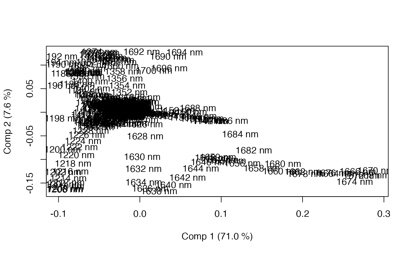
# Use of labels in plots and x scales
data(gasoline)
colnames(gasoline$NIR) <- paste(seq(900, 1700, 2), "nm")
gas <- plsr(octane ~ NIR, ncomp = 10, data = gasoline)
loadingplot(gas, labels="numbers")

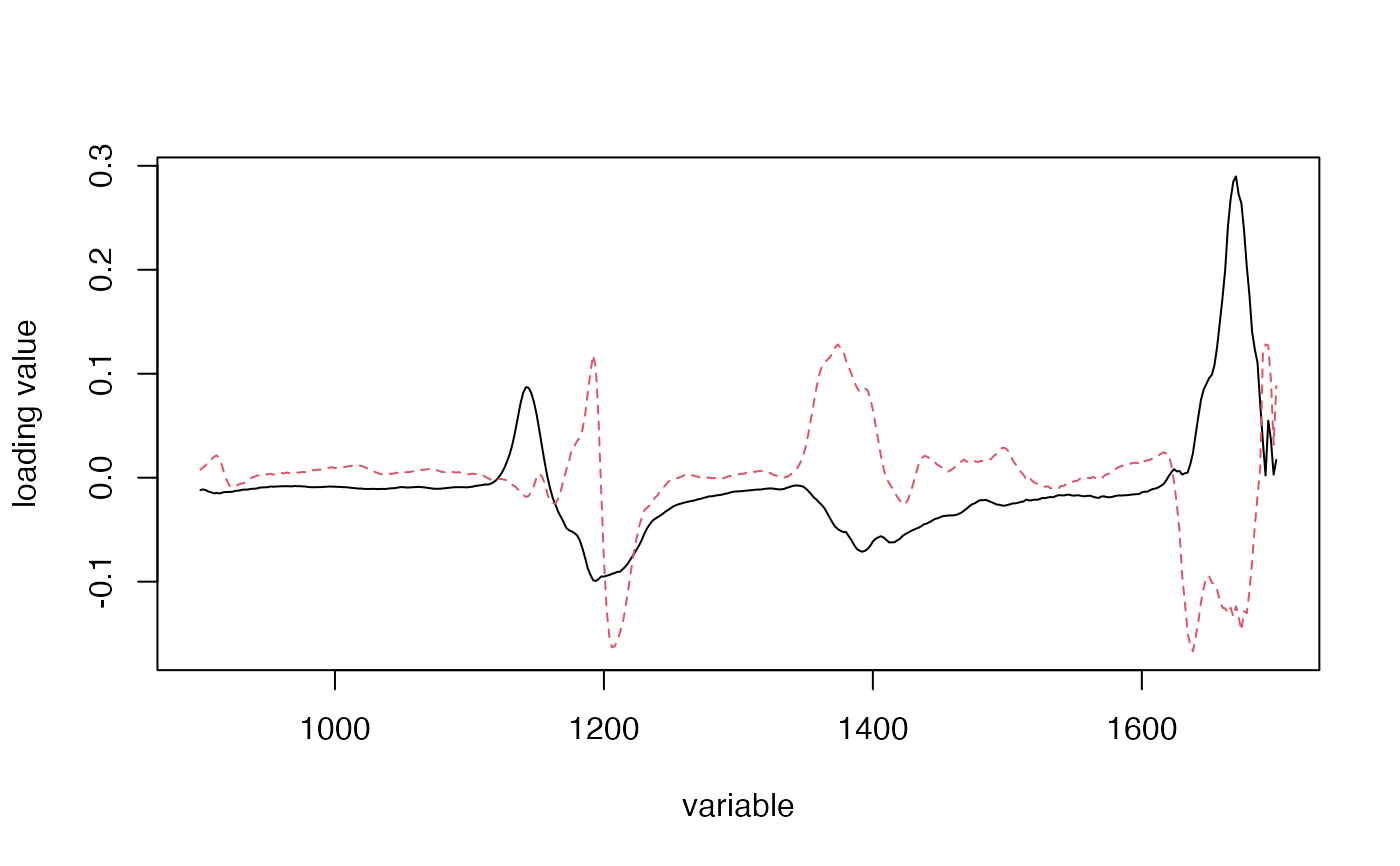loadingplot(gas, labels="names")

loadingplot(gas, labels="names", scatter=TRUE)